Chapter 4 Methods
The current study investigates the performance of the different model reduction processes using a Monte Carlo simulation. The simulation will be designed to follow the structure and characteristics of the DTMR data and the corresponding estimated parameters.
4.1 Overview of Monte Carlo methods
Broadly speaking, Monte Carlo simulations can be used to evaluate the performance of different or competing methodologies (Rubinstein & Kroese, 2017). As discussed in section 3.3, when using real data it is difficult to evaluate competing procedures, because the true values of the parameters are unknown. Thus, the estimates from different procedures can be compared to each other, but cannot be compared to what the real value is. With Monte Carlo methods, data is generated from a model with known parameters. The different procedures can be used on the simulated data, and then the resulting estimates compared to the actual values that were used to generate the data.
The general process of a Monte Carlo simulation is as follows:
- Define distributions for model parameters,
- Randomly draw model parameters from previously defined distributions,
- Simulate response data from the drawn model parameters,
- Estimate the model using simulated response data, and
- Compare estimated parameters to the parameters that were randomly drawn and used to simulate the data.
Monte Carlo studies have been used extensively in psychometric research (see Feinberg & Rubright, 2016 for a survey of simulation studies in educational measurement). There are disadvantages to this methodology however (e.g., Harwell, Stone, Hsu, & Kirisci, 1996). In the simulation of data, only parameters that are defined influence the generation of response data. Thus, if the model specified in the simulation study is inconsistent with reality, the simulation may not be informative. Additionally, the data generated will be perfectly model fitting (unless misfit is introduced in the data generation process). This means that the findings of the simulation study may not hold when there is misfit in the data. In other words, the main disadvantage of Monte Carlo studies is that simulation environment may not generalize to empirical data. Therefore, when designing a Monte Carlo study it is important to make the conditions and parameter distributions as realistic as possible (Feinberg & Rubright, 2016).
4.2 The current simulation
In order to make this simulation as realistic as possible, it will be modeled after the DTMR assessment and the results from the pilot study.
4.2.1 Simulation conditions
The DTMR assessment consists of 28 items measuring four attributes. The simulation study will use three and four attributes in order to assess the effects of increasingly complex structural models. Additionally, each condition will hold the number of items constant at 30 to reduce the number of conditions in the simulation. Three sample size conditions will be used: 500, 1000, and 5000. These sizes are representative of hte DTMR sample size of 990, a smaller sample, and a large sample that would remove any sample size concerns for estimation. This will allows for the evaluation of sample size effects. Thus, there are two attribute conditions times three sample size conditions = six data generation conditions.
For each generated data set, three Q-matrices will be used to estimate the model: the true Q-matrix, a 10 percent over-specified Q-matrix, and a 20 percent over-specified Q-matrix. In the over-specified Q-matrices, each value of zero in the Q-matrix will have either a 10 or 20 percent chance of being changed to a one, depending on the condition. Finally, for each Q-matrix, the model will be estimated in six ways:
- Saturated model,
- Simultaneous reduction,
- Measurement reduction,
- Structural reduction,
- Measurement-Structural reduction, and
- Structural-Measurement reduction.
This results in a total of three Q-matrix conditions times six model estimation conditions = 18 estimation conditions. Therefore, there are six data generation conditions times 18 estimation conditions = 108 total conditions. Each condition will be replicated 100 times to ensure that robust estimates of the outcomes measures can be calculated for each condition.
4.2.2 Data generation process
When simulating data sets, the \(\gamma\) parameters that make up the structural model will be simulated first. There are no constraints on the values of \(\gamma\); however, based on the results of the pilot study, structural parameters will be drawn from a \(\mathcal{N}(0, 2)\) distribution. Using this distribution, most draws will come within 3 standard deviations of the mean, resulting in most values falling between -6 and 6. These values are consistent with what is seen in the DTMR pilot study (Table 3.11). Additionally, this range allows for large effects using the guidelines suggest by Chinn (2000), but also makes very large \(\gamma\) values unlikely.
Once the structural parameters have been generated, the base rate probabilities for each class can be calculated. These will in turn be used to generate attribute profiles for the simulated respondents. The attribute profiles, in conjunctions with item parameters, are used to calculate the probability of each respondent answering each item correctly. The item intercepts will be drawn from a uniform distribution of [-5.00, 0.60]. This range is representative of the intercepts found in the pilot study, which range from -5.03 to 0.60 (Table 3.2), and therefore provides a realistic distribution of possible values. The main effects of the LCDM are constrained to be positive. Thus, these parameters will be drawn from of uniform distribution of (0.00, 5.00]. This is also based on the results on the pilot study, where the large estimated main effect was 5.19 (Table 3.3, Table 3.4, Table 3.5, and Table 3.6). Finally, the interaction terms are bounded on the lower end by \(-1 \times smallest\ main\ effect\). Thus the distribution for each interaction will be dependent on the main effects that are generated, but will all be bound on the upper end at 2.00. Only one interaction term from the pilot study fell beyond this range, the interaction between attributes 1 (RU) and 4 (MC) for item 13 in the structural reduction condition (Table 3.8). The item parameters and the attribute profiles are then used to calculate the probability of each respondent answering each item correctly. For each respondent/item combination then, a random uniform number is drawn between 0 and 1. If this random number is less than the probability of the respondent providing a correct response, a correct response is assigned (1), otherwise and incorrect response is assigned (0).
4.2.3 Model reduction process
Due to the potential issue in the convergence of DCMs noted in section 2.5.3, model reduction may occur in one of two ways for this study. The first method is used for the reduction of models that successfully converged. Given a converged model, parameters to remove are identified by their p-values, as was the case for analysis of the DTMR assessment (Chapter 3). The second method is for models that did not successfully converge. In this scenario, because p-values cannot be used to determine parameters that should be removed, all higher-order interaction parameters are flagged for removal (i.e., three-way interactions and greater). This heuristic is implemented in this study for two main reasons. First, it is highly unlikely that after collecting data, a researcher would simply give up on estimating the model if the fully saturated model did not converge. Thus, the inclusion of this rule-based model reduction will inform practitioners on best practices. Secondly, the removal of higher-order interaction terms has already been implemented in the literature as a method for dealing with non-convergence (see Bradshaw et al., 2014 for an example). Accordingly, this implementation of this rule in the simulation study mimics the current practice of model estimation. A modifiied model reduction flow chart can be seen in Figure 4.1.
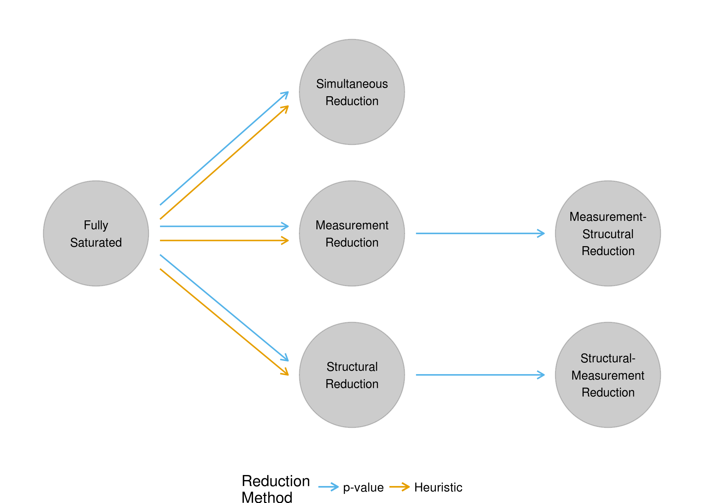
Figure 4.1: Flowchart of simulation study reduction processes
Note that in Figure 4.1, the rule-based model reductions can only occur after the fully saturated model. The logic behind this decision is as follows. If the fully saturated converges and the next model fails to converge, the practitioner should revert back to the model that successfully converged, rather than continuing to attempt to remove additional parameters. Conversely, if the fully saturated model fails to converge, and the next model also fails to converge, then the third model would result in the removal of both measurement and structural parameters using the heuristic. This would then be equivalent to the simultaneous reduction method using the heuristic, rendering third-step model redundant. Finally, regardless of the convergance of the fully saturated model, if the second-step model converges, the model reduction process can continue to the third step using p-values.
4.2.4 Outcome measures
Results for models that were reduced from converged and non-converged models will be analyzed separately. This is to allow for the possibility that different methods of reducing the model may prefer different model reduction processes. Accordingly, convergence rates of each model reduction process will be an important outcome measure. In addition, estimated item and structural parameters will be compared to the true values. The bias and mean squared error of the estimates will be calculated to evaluate the ability of each model reduction process to recover the parameter values. In these calculations, parameters that were removed in the reduction process will have their estimates set to 0.
In addition to the recovery of model parameters, the recovery of attribute profiles will also be examined. This will be calculated at both the attribute and pattern level. This distinction differentiates how accurate attribute mastery was and how accurate profile assignment was. For example, assume a respondent had a true attribute profile of [1,0,1,0], and an estimated profile of [1,1,1,0]. At the pattern level, they were incorrectly assigned to an attribute profile. However, at the attribute level, 75% of attributes were correctly estimated. These measures will be evaluated using percent correct classification, and the quadratically weighted Cohen’s kappa (Cohen, 1960, 1968).
Another important outcome of the model fitting process is model data fit. Thus, it is important to investigate whether any reduction processes consistently provide better fit to the data. This will be assessed using the Akaike information criterion (AIC; Akaike, 1974), Bayesian information criterion (BIC; Schwarz, 1978), and the adjusted Bayesian information criterion (Sclove, 1987). These methods all measure the relative fit of a model compared to competing models. All the methods measure how well the model fits the data, with a penalty for the number of parameters. Within each measure, the model with the lowest index on the measure is the preferred model, taking into account both overall fit and model complexity.
Finally, diagnostics of the model reduction processes will be examined. Specifically, the rate at which each process results in the correct parameters being retained in the model will be examined. This will be examined separately for the measurement and structural models. Additionally, the distributions of the values and standard errors of parameters that are reduced with p-values will be evaluated. This will allow for an analysis of whether reduced parameters are being removed due to small parameter estimates or overly large standard errors.
4.2.5 Software
As with the pilot study, all models were estimated using Mplus version 7.4 (L. K. Muthén & Muthén, 1998) via the MplusAutomation package (Hallquist & Wiley, 2018) in R version 3.4.4 (R Core Team, 2017). Mplus code for the estimation of the LCDM was generated in R using custom scripts based on the work of Rupp & Wilhelm (2012) and Templin & Hoffman (2013). Data generation and evaluation of the models was carried out in R using the dplyr (Wickham, François, Henry, & Müller, 2018), forcats (Wickham, 2018a), glue (Hester, 2017), lubridate (Spinu, Grolemund, & Wickham, 2018), portableParallelSeeds (Johnson, 2016), purrr (Henry & Wickham, 2017), readr (Wickham, Hester, & Francois, 2017), stringr (Wickham, 2018b), tibble (Müller & Wickham, 2018), tidyr (Wickham & Henry, 2018), and tidyselect (Henry & Wickham, 2018) packages. All analyses were carried out on the Amazon Elastic Compute Cloud (EC2; Amazon Web Services, 2018).