Chapter 3 Pilot Study
In order to better assess the impact of the order of model reduction, a pilot study was conducted on the Diagnosing Teachers’ Multiplicative Reasoning (DTMR) assessment data, as described in Bradshaw et al. (2014). In this study, the DTMR data set was analyzed using a variety of model reduction processes to determine if the selected process has an impact on the resulting model parameters. Thus, the pilot study was designed to answer the first research question defined in section 2.6. This is an important first step as without evidence that the model reduction process has an impact on the results, there would be little motivation for a more thorough analysis via simulation.
3.1 Method
3.1.1 DTMR data
The DTMR assessment consists of 28 dichotomously scored items that together measure 4 attributes related to educators’ understanding of multiplicative reasoning (Bradshaw et al., 2014):
- Referent Units (RU): recognizing which whole the fraction refers to,
- Partitioning and Iterating (PI): splitting a whole into equal pieces repeatedly to achieve larger fractions,
- Appropriateness (APP): determining the correct mathematical operation from a problem statement, and
- Multiplicative Comparison (MC): evaluating the ratio of one value to another.
Of the 28 items, Referent Units is measured by 16, Partitioning and Iterating by 10, Appropriateness by 6, and Multiplicative Comparison by 10. This totals adds to more than 28 because several items measure more than one attribute. Specifically, there are 14 items measuring only 1 attribute and 14 that measure 2 attributes. The complete saturated Q-matrix for the DTMR assessment can be see in Table 3.1. For example, item 1 measures only the Referent Units attribute, whereas item 5 measures both the Referent Units and Multiplicative Comparison attributes.
| Item | Item Name | RU | PI | APP | MC |
|---|---|---|---|---|---|
| 1 | 1 | 1 | 0 | 0 | 0 |
| 2 | 2 | 0 | 0 | 1 | 0 |
| 3 | 3 | 0 | 1 | 0 | 0 |
| 4 | 4 | 1 | 0 | 0 | 0 |
| 5 | 5 | 1 | 0 | 0 | 1 |
| 6 | 6 | 0 | 1 | 0 | 0 |
| 7 | 7 | 1 | 0 | 0 | 0 |
| 8 | 8a | 0 | 0 | 1 | 1 |
| 9 | 8b | 0 | 0 | 1 | 0 |
| 10 | 8c | 0 | 0 | 1 | 0 |
| 11 | 8d | 0 | 0 | 1 | 0 |
| 12 | 9 | 1 | 0 | 0 | 0 |
| 13 | 10a | 1 | 0 | 0 | 1 |
| 14 | 10b | 1 | 0 | 0 | 1 |
| 15 | 10c | 1 | 0 | 0 | 1 |
| 16 | 11 | 1 | 0 | 0 | 1 |
| 17 | 12 | 1 | 0 | 0 | 0 |
| 18 | 13 | 0 | 1 | 0 | 1 |
| 19 | 14 | 1 | 1 | 0 | 0 |
| 20 | 15a | 0 | 1 | 0 | 1 |
| 21 | 15b | 0 | 1 | 0 | 1 |
| 22 | 15c | 0 | 1 | 0 | 1 |
| 23 | 16 | 1 | 0 | 0 | 0 |
| 24 | 17 | 1 | 1 | 0 | 0 |
| 25 | 18 | 1 | 1 | 0 | 0 |
| 26 | 19 | 0 | 0 | 1 | 0 |
| 27 | 21 | 1 | 0 | 0 | 0 |
| 28 | 22 | 1 | 1 | 0 | 0 |
In total 990 math teachers took the assessment. Bradshaw et al. (2014) reported that sample demographics were consistent with a representative national sample. For a complete description of the sample characteristics and data collection process, see the original description of the DTMR in Bradshaw et al. (2014).
3.1.2 Model estimation
In order to assess the impact of various model reduction processes, the LCDM was estimated for the DTRM using five different reduction methods:
- Simultaneous reduction: after estimating the fully saturated model, all non-significant parameters from both the measurement and the structural models are removed and the model is re-estimated,
- Measurement reduction: after estimating the fully saturated model, all non-significant parameters from the measurement model only are removed and the model is re-estimated,
- Structural reduction: after estimating the fully saturated model, all non-significant parameters from the structural model only are removed and the model is re-estimated,
- Measurement-Structural reduction: after estimating the measurement reduction model, all non-significant parameters from the structural model only are removed and the model is re-estimated, and
- Structural-Measurement reduction: after estimating the structural reduction model, all non-significant parameters from the measurement model only are removed and the model is re-estimated.
The different ordering processes for model reduction, and their relationships to each other, are represented visually in Figure 3.1. The significance of each parameter was determined by the p-value derived from the Wald test provided by Mplus. This test provides a p-value for the null hypothesis that the parameter is equal to zero. Parameters with a p-value greater than 0.05 were determined to be non-significant, and therefore removed at the corresponding stage of model reduction. It should be noted that in the model reduction processes outlined, a constraint was put in place to prevent the removal of item intercepts. An intercept must be defined in order to ensure that all respondents have an estimated probability of a correct response. Thus, item intercepts remained in the model, regardless of their significance.
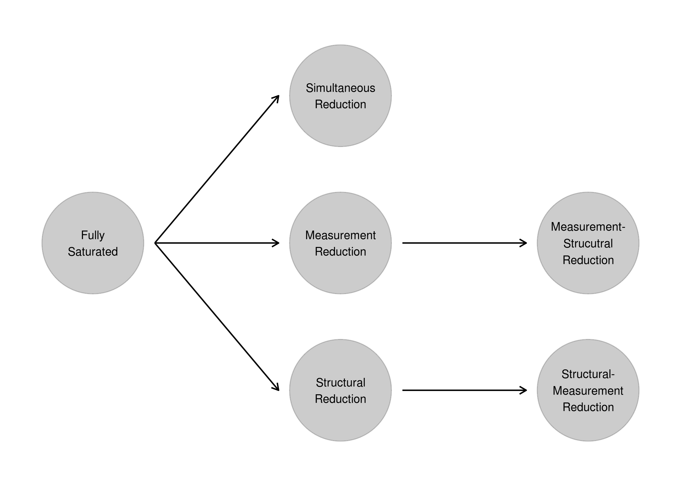
Figure 3.1: Flowchart of model reduction processes
In practical terms, a non-significant intercept means that the log-odds of a respondent who hasn’t mastered any of the required attributes is not significantly different from 0 (this corresponds to a probability of 0.5). Thus, these cases may represent easier, or highly guessable items, where non-masters of the required traits still have a relatively high probability of success. In contrast, non-significant main effects and interactions represent instances where the increase in the log-odds for masters of the given attribute (or combination of attributes in the case of interactions) is not significantly different from 0. Thus, after removing these parameters, the affected respondents would have the same probability of providing a correct response as respondents who had not mastered the required attributes. In the extreme case where all parameters for an item are removed except for the intercept, all respondents would have the same probability of success, regardless of their profile of attribute mastery.
All analyses for the pilot study were conducted in Mplus version 7.4 (L. K. Muthén & Muthén, 1998) via the MplusAutomation package (Hallquist & Wiley, 2018) in R version 3.4.4 (R Core Team, 2017). Mplus code for the estimation of the LCDM was generated in R using custom scripts based on the work of Rupp & Wilhelm (2012) and Templin & Hoffman (2013).
3.2 Results
The final estimate and associated standard error for each parameter from each of the model reduction processes are presented in their own tables in order to easily compare across model reduction processes. Table 3.2, Table 3.3, Table 3.4, Table 3.5, Table 3.6, Table 3.7, Table 3.8, Table 3.9, and Table 3.10 show the results of the measurement model parameters, and Table 3.11 shows the results of the structural model parameters.
| Item | Simultaneous Reduction | Measurement Reduction | Structural Reduction | Measurement-Structural Reduction | Structural-Measurement Reduction |
|---|---|---|---|---|---|
| 1 | -1.11 (0.11) | -1.11 (0.03) | -1.10 (0.12) | -1.25 (0.15) | -1.10 (0.13) |
| 2 | 0.55 (0.13) | 0.59 (0.15) | 0.57 (0.13) | 0.60 (0.13) | 0.56 (0.14) |
| 3 | -1.98 (0.17) | -1.96 (0.06) | -2.17 (0.28) | -1.94 (0.18) | -2.03 (0.20) |
| 4 | -1.20 (0.10) | -1.20 (14.55) | -1.19 (0.11) | -1.26 (0.12) | -1.20 (0.11) |
| 5 | -1.64 (0.12) | -1.65 (14.31) | -1.77 (0.19) | -1.78 (0.15) | -1.62 (0.14) |
| 6 | -3.84 (0.43) | -3.84 (0.26) | -3.90 (0.67) | -3.79 (0.43) | -3.80 (0.46) |
| 7 | -0.75 (0.09) | -0.76 (0.40) | -0.70 (0.09) | -0.78 (0.10) | -0.74 (0.09) |
| 8 | -0.57 (0.14) | -0.62 (0.11) | -0.74 (0.26) | -0.73 (0.31) | -0.59 (0.24) |
| 9 | -0.07 (0.13) | -0.09 (0.10) | -0.10 (0.19) | -0.15 (0.19) | -0.08 (0.17) |
| 10 | 0.29 (0.13) | 0.30 (0.02) | 0.28 (0.13) | 0.31 (0.13) | 0.28 (0.13) |
| 11 | -1.12 (0.16) | -1.03 (0.14) | -1.07 (0.17) | -0.99 (0.17) | -1.09 (0.17) |
| 12 | -1.23 (0.10) | -1.23 (0.10) | -1.21 (0.10) | -1.24 (0.11) | -1.24 (0.10) |
| 13 | -0.46 (0.14) | -0.51 (0.17) | -0.58 (0.19) | -0.44 (0.19) | -0.58 (0.21) |
| 14 | -3.86 (0.63) | -4.03 (0.57) | -3.61 (0.83) | -3.90 (0.67) | -4.01 (0.81) |
| 15 | -4.88 (0.89) | -4.92 (0.43) | -4.54 (0.78) | -5.03 (0.97) | -4.74 (0.89) |
| 16 | -0.87 (0.09) | -0.87 (0.06) | -0.99 (0.15) | -0.92 (0.11) | -0.86 (0.10) |
| 17 | -1.35 (0.11) | -1.37 (0.10) | -1.25 (0.11) | -1.44 (0.12) | -1.33 (0.11) |
| 18 | -0.24 (0.07) | -0.24 (15.05) | -0.77 (0.18) | -0.24 (0.07) | -0.24 (0.07) |
| 19 | -1.52 (0.08) | -1.52 (11.98) | -2.17 (0.35) | -1.52 (0.08) | -1.52 (0.08) |
| 20 | -1.85 (0.18) | -1.84 (0.01) | -2.47 (0.37) | -1.72 (0.20) | -2.49 (0.29) |
| 21 | -0.37 (0.12) | -0.32 (0.16) | -0.68 (0.24) | -0.27 (0.13) | -0.46 (0.16) |
| 22 | -0.26 (0.12) | -0.23 (0.11) | -0.61 (0.22) | -0.17 (0.13) | -0.55 (0.18) |
| 23 | -0.89 (0.10) | -0.89 (13.43) | -0.85 (0.10) | -0.92 (0.10) | -0.89 (0.10) |
| 24 | -2.09 (0.19) | -2.06 (0.06) | -2.14 (0.28) | -1.98 (0.18) | -2.04 (0.22) |
| 25 | -0.95 (0.12) | -0.92 (0.06) | -0.98 (0.14) | -0.88 (0.12) | -0.99 (0.14) |
| 26 | -2.49 (0.12) | -2.49 (0.12) | -2.49 (0.12) | -2.49 (0.12) | -2.49 (0.12) |
| 27 | -1.46 (0.11) | -1.47 (0.29) | -1.48 (0.12) | -1.59 (0.14) | -1.47 (0.13) |
| 28 | -1.19 (0.13) | -1.17 (0.21) | -1.29 (0.18) | -1.17 (0.14) | -1.24 (0.15) |
| * Parentheses show the standard error of the estimate. |
| Item | Simultaneous Reduction | Measurement Reduction | Structural Reduction | Measurement-Structural Reduction | Structural-Measurement Reduction |
|---|---|---|---|---|---|
| 1 | 2.19 (0.20) | 2.19 (0.13) | 2.22 (0.21) | 2.11 (0.19) | 2.20 (0.20) |
| 4 | 0.66 (0.18) | 0.67 (0.42) | 0.64 (0.19) | 0.70 (0.18) | 0.67 (0.19) |
| 5 | 1.45 (0.19) | 1.47 (0.28) | 1.51 (0.65) | 1.51 (0.20) | 1.43 (0.20) |
| 7 | 1.26 (0.19) | 1.30 (0.38) | 1.15 (0.22) | 1.12 (0.20) | 1.25 (0.23) |
| 12 | 0.78 (0.18) | 0.78 (0.11) | 0.74 (0.20) | 0.68 (0.18) | 0.81 (0.19) |
| 13 | 2.55 (0.94) | 0.89 (0.62) | |||
| 14 | 1.31 (0.27) | 1.33 (0.11) | 3.79 (1.28) | 1.19 (0.30) | 1.49 (0.32) |
| 15 | 1.12 (0.24) | 1.16 (0.10) | 4.19 (1.07) | 1.07 (0.27) | 0.00 (0.00) |
| 16 | 1.22 (0.17) | 1.23 (0.12) | 1.36 (0.20) | 1.15 (0.17) | 1.23 (0.18) |
| 17 | 2.04 (0.20) | 2.08 (0.12) | 1.82 (0.21) | 1.89 (0.20) | 2.01 (0.23) |
| 19 | 0.20 (1.53) | ||||
| 23 | 1.61 (0.21) | 1.62 (0.28) | 1.54 (0.23) | 1.41 (0.21) | 1.65 (0.25) |
| 24 | 0.24 (0.34) | ||||
| 25 | 1.06 (0.70) | ||||
| 27 | 1.59 (0.19) | 1.60 (0.37) | 1.66 (0.20) | 1.60 (0.19) | 1.63 (0.19) |
| 28 | 1.22 (0.29) | 1.20 (0.12) | 2.59 (0.86) | 1.08 (0.33) | 1.36 (0.30) |
| * Parentheses show the standard error of the estimate. | |||||
| † Missing values indicate the parameter was removed in the reduction process. |
| Item | Simultaneous Reduction | Measurement Reduction | Structural Reduction | Measurement-Structural Reduction | Structural-Measurement Reduction |
|---|---|---|---|---|---|
| 3 | 1.65 (0.21) | 1.65 (0.03) | 1.90 (0.33) | 1.67 (0.21) | 1.69 (0.23) |
| 6 | 2.18 (0.47) | 2.20 (0.23) | 2.23 (0.74) | 2.18 (0.46) | 2.11 (0.49) |
| 18 | 0.52 (0.38) | ||||
| 19 | 0.08 (1.02) | ||||
| 20 | 3.05 (0.24) | 3.11 (0.09) | 2.52 (0.54) | 3.05 (0.24) | 2.69 (0.26) |
| 21 | 2.69 (0.24) | 2.64 (0.10) | 1.98 (0.68) | 2.69 (0.28) | 2.87 (0.29) |
| 22 | 2.83 (0.27) | 2.82 (0.09) | 2.03 (0.65) | 2.88 (0.33) | 2.73 (0.33) |
| 24 | 2.04 (0.23) | 2.03 (0.05) | 1.45 (0.42) | 1.97 (0.21) | 1.36 (0.33) |
| 25 | 1.74 (0.17) | 1.70 (0.06) | 1.16 (0.27) | 1.72 (0.17) | 1.77 (0.18) |
| 28 | 1.56 (0.24) | 1.56 (0.17) | 1.64 (0.30) | 1.55 (0.29) | 1.54 (0.25) |
| * Parentheses show the standard error of the estimate. | |||||
| † Missing values indicate the parameter was removed in the reduction process. |
| Item | Simultaneous Reduction | Measurement Reduction | Structural Reduction | Measurement-Structural Reduction | Structural-Measurement Reduction |
|---|---|---|---|---|---|
| 2 | 1.30 (0.20) | 1.27 (0.06) | 1.30 (0.22) | 1.22 (0.24) | 1.30 (0.21) |
| 8 | 3.63 (0.34) | 4.32 (0.11) | 4.20 (0.58) | 4.55 (0.68) | 3.83 (0.51) |
| 9 | 2.02 (0.21) | 2.16 (0.14) | 2.17 (0.25) | 2.24 (0.23) | 2.09 (0.25) |
| 10 | 0.84 (0.18) | 0.84 (0.04) | 0.88 (0.18) | 0.81 (0.18) | 0.87 (0.18) |
| 11 | 1.89 (0.20) | 1.81 (0.19) | 1.86 (0.24) | 1.72 (0.21) | 1.86 (0.21) |
| 26 | 0.00 (0.00) | ||||
| * Parentheses show the standard error of the estimate. | |||||
| † Missing values indicate the parameter was removed in the reduction process. |
| Item | Simultaneous Reduction | Measurement Reduction | Structural Reduction | Measurement-Structural Reduction | Structural-Measurement Reduction |
|---|---|---|---|---|---|
| 5 | 0.27 (0.31) | ||||
| 8 | 0.54 (0.50) | ||||
| 13 | 4.87 (0.60) | 4.89 (2.00) | 5.19 (2.08) | 4.87 (0.60) | 4.47 (0.56) |
| 14 | 4.13 (0.66) | 4.28 (0.64) | 3.80 (0.84) | 4.12 (0.65) | 4.21 (0.81) |
| 15 | 4.66 (0.91) | 4.67 (0.46) | 4.19 (0.81) | 4.75 (0.96) | 4.44 (0.91) |
| 16 | 0.25 (0.25) | ||||
| 18 | 0.48 (0.28) | ||||
| 20 | 1.25 (0.50) | 1.22 (0.28) | |||
| 21 | 0.63 (0.36) | ||||
| 22 | 0.83 (0.34) | 0.52 (0.27) | |||
| * Parentheses show the standard error of the estimate. | |||||
| † Missing values indicate the parameter was removed in the reduction process. |
| Item | Simultaneous Reduction | Measurement Reduction | Structural Reduction | Measurement-Structural Reduction | Structural-Measurement Reduction |
|---|---|---|---|---|---|
| 19 | 1.35 (1.95) | ||||
| 24 | 0.91 (0.43) | 1.04 (0.27) | |||
| 25 | 0.04 (0.84) | ||||
| 28 | -1.36 (0.94) | ||||
| * Parentheses show the standard error of the estimate. | |||||
| † Missing values indicate the parameter was removed in the reduction process. |
| Item | Simultaneous Reduction | Measurement Reduction | Structural Reduction | Measurement-Structural Reduction | Structural-Measurement Reduction |
|---|---|---|---|---|---|
| 5 | -0.16 (0.88) | ||||
| 13 | 3.65 (6.32) | ||||
| 14 | -1.93 (1.57) | ||||
| 15 | -2.45 (1.14) | 1.32 (0.28) | |||
| 16 | -0.25 (0.25) | ||||
| * Parentheses show the standard error of the estimate. | |||||
| † Missing values indicate the parameter was removed in the reduction process. |
| Item | Simultaneous Reduction | Measurement Reduction | Structural Reduction | Measurement-Structural Reduction | Structural-Measurement Reduction |
|---|---|---|---|---|---|
| 18 | -0.04 (0.47) | ||||
| 20 | 0.79 (0.71) | ||||
| 21 | 1.95 (2.27) | ||||
| 22 | 1.54 (1.46) | ||||
| * Parentheses show the standard error of the estimate. | |||||
| † Missing values indicate the parameter was removed in the reduction process. |
| Item | Simultaneous Reduction | Measurement Reduction | Structural Reduction | Measurement-Structural Reduction | Structural-Measurement Reduction |
|---|---|---|---|---|---|
| 8 | -0.54 (0.50) | ||||
| * Parentheses show the standard error of the estimate. | |||||
| † Missing values indicate the parameter was removed in the reduction process. |
3.2.1 Measurement model results
Although it is tempting to compare the point estimates and standard errors for the parameters across model reduction techniques, this is ill-advised. Because the main effects and interactions are conditional on other parameters in the model, the exclusion of parameters will change the interpretation of the other parameters. Thus, changes in point estimates and standard errors may be expected. Thus, these results are most useful for comparing which parameters are ultimately retained in the model. In general we can see that the choice of the model reduction method can have a profound impact on which parameters are ultimately retained in the model. The exception to this is the item intercepts (Table 3.2). Because model reduction was constrained to never remove item intercepts, all intercepts are estimated, no matter which reduction technique was used. This is not the case for main effects. For example, when examining the main effects for attribute 1 (Table 3.3), the main effect for item 13 was only retained when either the structural model only was reduced, or when the structural model was reduced first. This is because when the measurement model was reduced first, this main effect was non-significant, and thus reduced out of the model. However, reduction of the structural model first changed the parameter estimate and associated p-value enough for the parameter to be significant, and thus retained.
A similar, but more extreme pattern can be seen in the interactions in the measurement model (Tables 3.7, 3.8, 3.9, 3.10). Interactions between the attributes were only retained when the structural model alone was reduced (in which case all interactions from the measurement model were kept) or when the structural model was reduced first (in which case some of the interactions were retained). If the measurement model was reduced before the structural model, or with the structural model simultaneously, interaction terms from the measurement model were never retained.
Finally, as mentioned above, it is generally ill-advised to compare point estimates and standard errors across model reduction methods. The exception to this rule is the item intercepts, because these parameters are not dependent on the other terms in the model (i.e., the intercept always represents the log-odds of providing a correct response when none of the attributes have been mastered). Thus, it is possible to compare these parameters across model reductions methods. It is clear that although these parameters are generally similar, the standard errors sometimes vary wildly (for example, Table 3.2). For instance, the standard error of the intercept on item four is consistently around 0.10, except for when only the measurement model is reduced. In this situation, the standard error is 14.55. A similar pattern can be seen in the intercepts for items 5, 18, 19, and 23.
3.2.2 Structural model results
The parameters of the structural model also show variability between model reduction processes. As with the measurement model parameters, different model reduction processes result in different parameters ultimately being retained in the model. Table 3.11 shows, for example, that 3-way interactions are almost always removed unless the measurement model is reduced first. The exception is the 3-way interaction between the Referent Units, Appropriateness, and Multiplicative Comparison attributes. Notably, this interaction appears to be relatively unstable across model reduction process, varying from 2.40 to 14.94. However, this variability in point estiamtes should be interpreted with caution. As was the case when examining the measurement model parameters, the structural parameters are also conditional upon other parameters, and thus, fluctuations may be expected depending on the inclusion or exclusion of the other parameters.
The variation in which strucutral parameters are ultimately retained in the model can have serious implications for classification of respondents. Given that these parameters govern the base rate probabilities of membership in each of the attribute profiles, these differences in included parameters could lead to differences in the classification of respondents.
| Parameter | Simultaneous Reduction | Measurement Reduction | Structural Reduction | Measurement-Structural Reduction | Structural-Measurement Reduction |
|---|---|---|---|---|---|
| \(\gamma_{1,(1)}\) | -5.11 (0.01) | -3.49 (1.58) | -10.06 (0.43) | -2.93 (0.62) | -6.85 (2.28) |
| \(\gamma_{1,(2)}\) | -2.10 (0.04) | -2.92 (1.17) | -1.65 (0.34) | -1.21 (0.24) | -1.80 (0.34) |
| \(\gamma_{1,(3)}\) | -1.54 (0.05) | -1.28 (0.35) | -1.40 (0.37) | -0.75 (0.33) | -1.55 (0.37) |
| \(\gamma_{1,(4)}\) | -1.06 (0.06) | -1.24 (0.13) | -0.84 (0.28) | -0.95 (0.24) | -0.91 (0.28) |
| \(\gamma_{2,(1,2)}\) | 3.44 (0.01) | -2.96 (0.04) | 8.75 (0.52) | -8.35 (0.66) | 5.56 (2.24) |
| \(\gamma_{2,(1,3)}\) | 0.53 (0.02) | -8.16 (3.62) | 1.53 (0.78) | -6.93 (0.68) | 0.36 (0.93) |
| \(\gamma_{2,(1,4)}\) | -5.24 (3.57) | ||||
| \(\gamma_{2,(2,3)}\) | 2.23 (0.02) | 2.46 (1.44) | 1.87 (0.46) | 2.02 (0.42) | |
| \(\gamma_{2,(2,4)}\) | 2.31 (1.34) | ||||
| \(\gamma_{2,(3,4)}\) | 1.89 (0.02) | 1.70 (0.34) | 1.51 (0.45) | 1.41 (0.36) | 1.81 (0.38) |
| \(\gamma_{3,(1,2,3)}\) | 13.91 (3.71) | 18.28 (0.78) | |||
| \(\gamma_{3,(1,2,4)}\) | 10.38 (3.60) | 10.79 (0.66) | |||
| \(\gamma_{3,(1,3,4)}\) | 2.40 (0.03) | 14.94 (0.12) | 7.15 (0.87) | 7.85 (0.70) | 4.73 (2.38) |
| \(\gamma_{3,(2,3,4)}\) | -1.65 (1.62) | ||||
| \(\gamma_{4,(1,2,3,4)}\) | -0.49 (0.03) | -18.66 (1.67) | -6.98 (0.68) | -16.70 (1.04) | -3.18 (2.34) |
| * Parentheses show the standard error of the estimate. | |||||
| † Missing values indicate the parameter was removed in the reduction process. |
Figure 3.2 shows the change in the number of respondents classified in each attribute profile under each model reduction processes. Although the counts are fairly consistent across most attribute profiles, the counts for profiles 15 ([0,1,1,1]) and 16 ([1,1,1,1]) do show large discrepancies. There are about 50 respondents classified as master of Partitioning and Iterating, Appropriateness, and Multiplicative Comparison under the measurement-structural reduction process, but around 150 when using all other processes. The attribute profile where all attributes is mastered ([1,1,1,1]) is even more volatile, with the number of respondents placed into this class varying from 200 to nearly 350 depending on the reduction method.
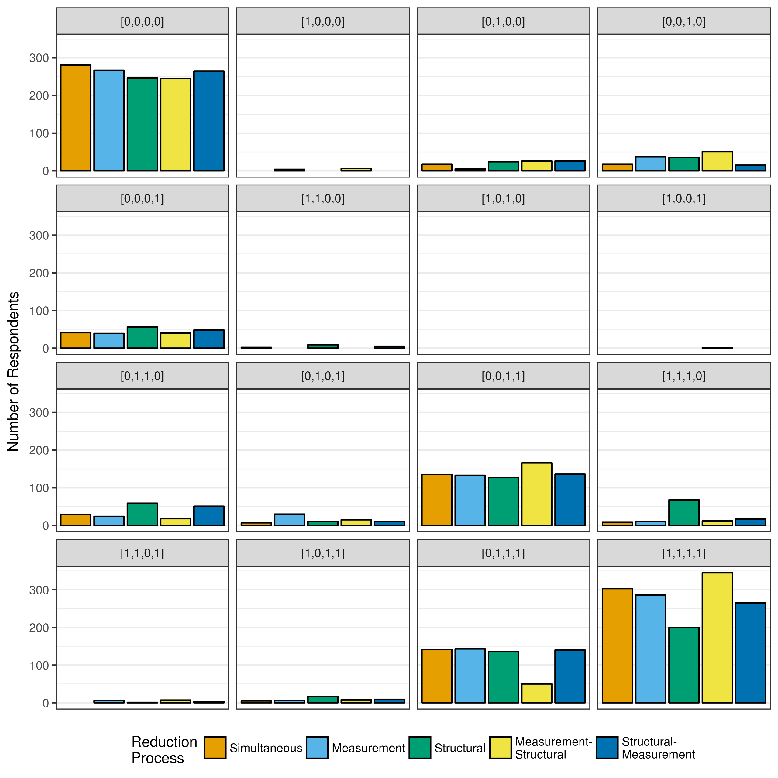
Figure 3.2: DTMR respondent classification under each model reduction process
3.3 Conclusions
The results from the pilot study provide evidence that the choice of model reduction process can significantly influence not only the estimates of the parameters, but also the classification of respondents into attribute profiles. However, without knowing the true values of parameters and attribute profiles of the respondents, it is impossible to know which model reduction process should be chosen. Therefore, a simulation study will be conducted in which the true values of the parameters and attribute profiles are known. In this way, it will be possible to measure how accurately each model reduction process is able to recover parameter values and respondent attribute profiles. The results of the simulation will then be able to inform which method is best suited to analyze the DTMR data.