Chapter 5 Results
Results from the simulation study are described in two sections. Section 5.1 summarizes the performance of the reduction processes when the parameters to reduce were determined by p-values from a converged model (i.e., p-value/p-value reduction). Section 5.2 summarizes results of the reduction processes for models that did not converge, and the parameters to reduce were determined by the higher order interaction heuristic (i.e., heuristic/p-value reduction).
Table 5.1 shows the convergence rates for the saturated model. As expected, the convergence rates decrease as the number of attributes increases, and decrease dramatically as the over specification of the Q-matrix increases. Interestingly, sample size had relatively little effect on the convergence rates of the saturated model, with rates staying fairly consistent with attribute and over specification conditions.
| Q-Matrix Over Specification | n = 500 | n = 1000 | n = 5000 | n = 500 | n = 1000 | n = 5000 |
|---|---|---|---|---|---|---|
| 0.0 | 0.85 | 0.76 | 0.87 | 0.69 | 0.67 | 0.64 |
| 0.1 | 0.31 | 0.49 | 0.43 | 0.07 | 0.09 | 0.11 |
| 0.2 | 0.09 | 0.05 | 0.11 | 0.01 | 0.01 | 0.02 |
5.1 Reduction by p-value
5.1.1 Convergence
When saturated model converged, reduction of measurement and structural parameters proceeded by using p-values to determine which parameters to reduce. Figure 5.1 shows the convergence rates for these reduction processes when the saturated model converged. Recall that measurement-structural and structural measurement reduction only occurred if the measurement and structural reductions, respectively, converged. Across all conditions, reduction processes where there measurement model was reduced first (i.e., simultaneous, measurement, and measurement-structural) tended to have higher convergence rates. This was most notable when the Q-matrix was over specified. In the most extreme case, the four-attribute condition with a 20 percent over specified Q-matrix, no reductions converged if the measurement model was not part of the initial reduction. However, because the saturated model very rarely converged for this condition (Table 5.1), the sample size is very limited.
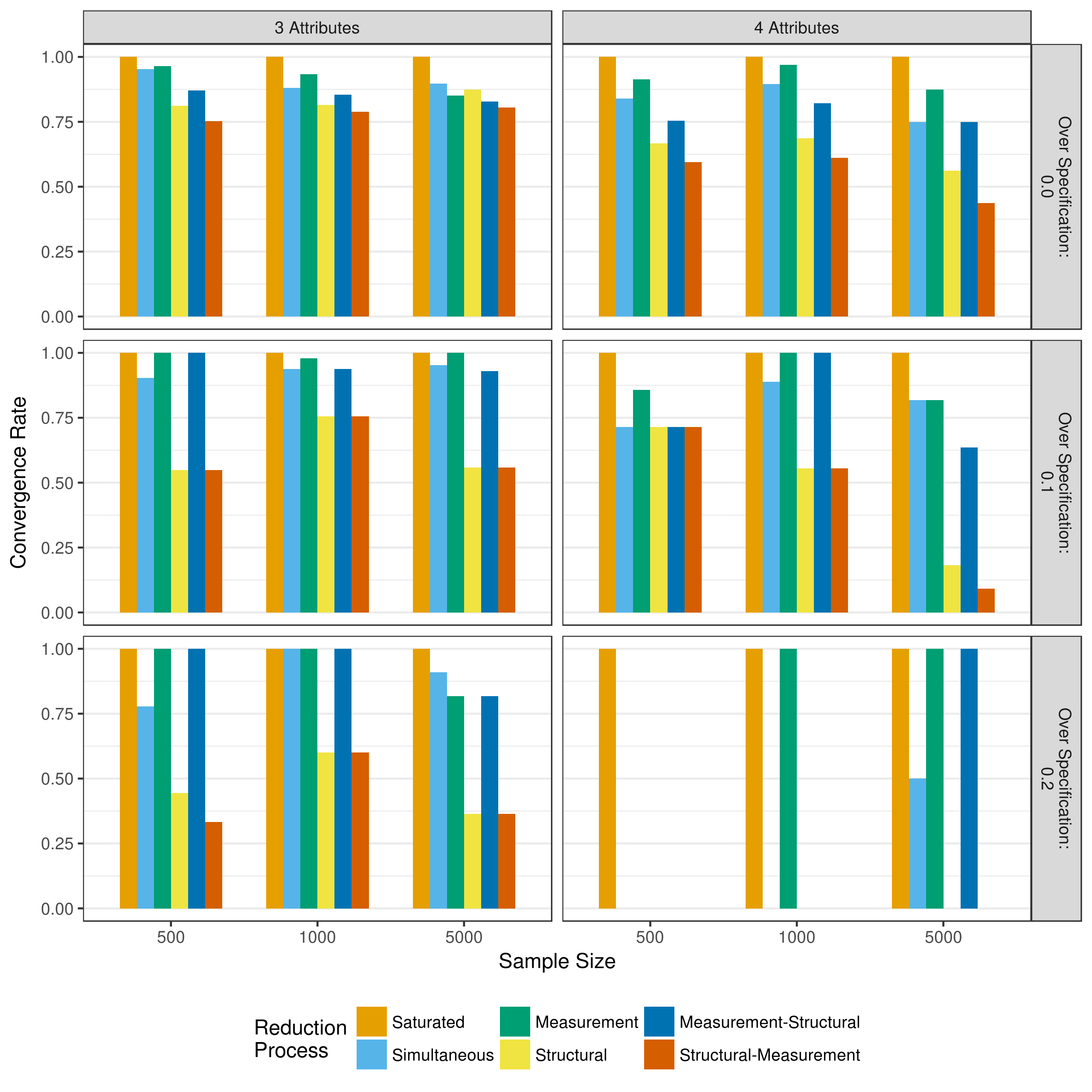
Figure 5.1: Convergence rates when reducing using p-values
5.1.2 Parameter recovery
To evaluate the performance of the reduction processes, the bias and mean square error of the parameter estimates can be examined. The bias represents the difference between the true value and the estimated value. The mean square error represents the average of the squared difference between the true and estimated values. Figure 5.2 and Figure 5.3 show the total bias and total mean square error, respectively, across all measurement model parameters when reducing using p-values. Because of some outlying data sets, biases with an absolute value greater than 100 and mean square errors with a value greater than 100 have been excluded from the figures. Figures showing all biases and mean square errors, separated by the type of parameter can be seen in Appendix A.
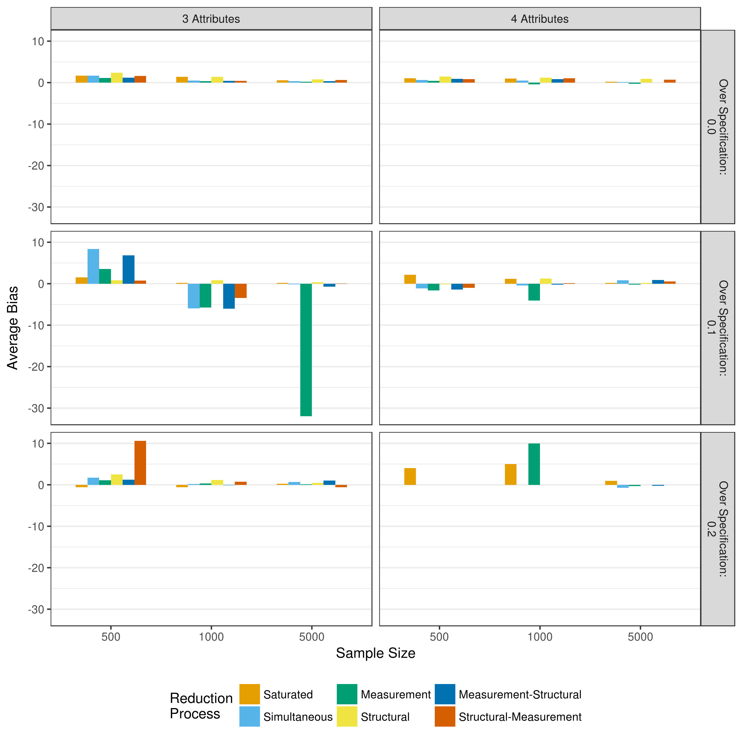
Figure 5.2: Bias in measurement model main effect estimates when reducing using p-values
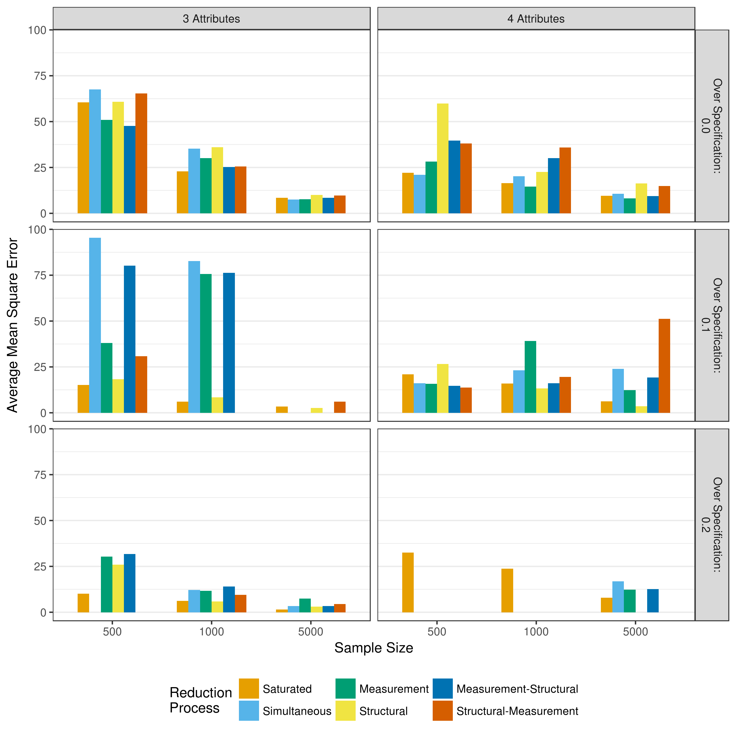
Figure 5.3: Mean square error in measurement model main effect estimates when reducing using p-values
Figure 5.2 shows that across all conditions there is relatively little bias in the measurement model parameters. This is especially true when the Q-matrix is correctly specified. The large negative bias seen in the measurement reduction condition for the three attribute and 10 percent over specified Q-matrix is due to a single three way interaction in one data set, as can be seen in Figure A.4. In contrast, there is relatively large mean square error values across conditions. As expected, this decreases as the sample size increases. Thus, these results suggest that larger sample sizes (i.e., greater than 1,000) are needed in order to ensure unbiased estimates of measurement model parameters with low levels of error.
Figure 5.4 and Figure 5.5 show the bias and mean square error of the structural parameters respectively. Overall, there is very little bias and mean squared error in the structural parameters. The instances where larger bias and mean squared error are indicated (e.g., measurement reduction of a four attribute model with a 20% over specified Q-matrix) are instances where very few of the model actually converged. Thus, these values are based on only a few replications. Thus, these results suggests that given model convergence, the structural parameters are usually well estimated regardless of model reduction method.
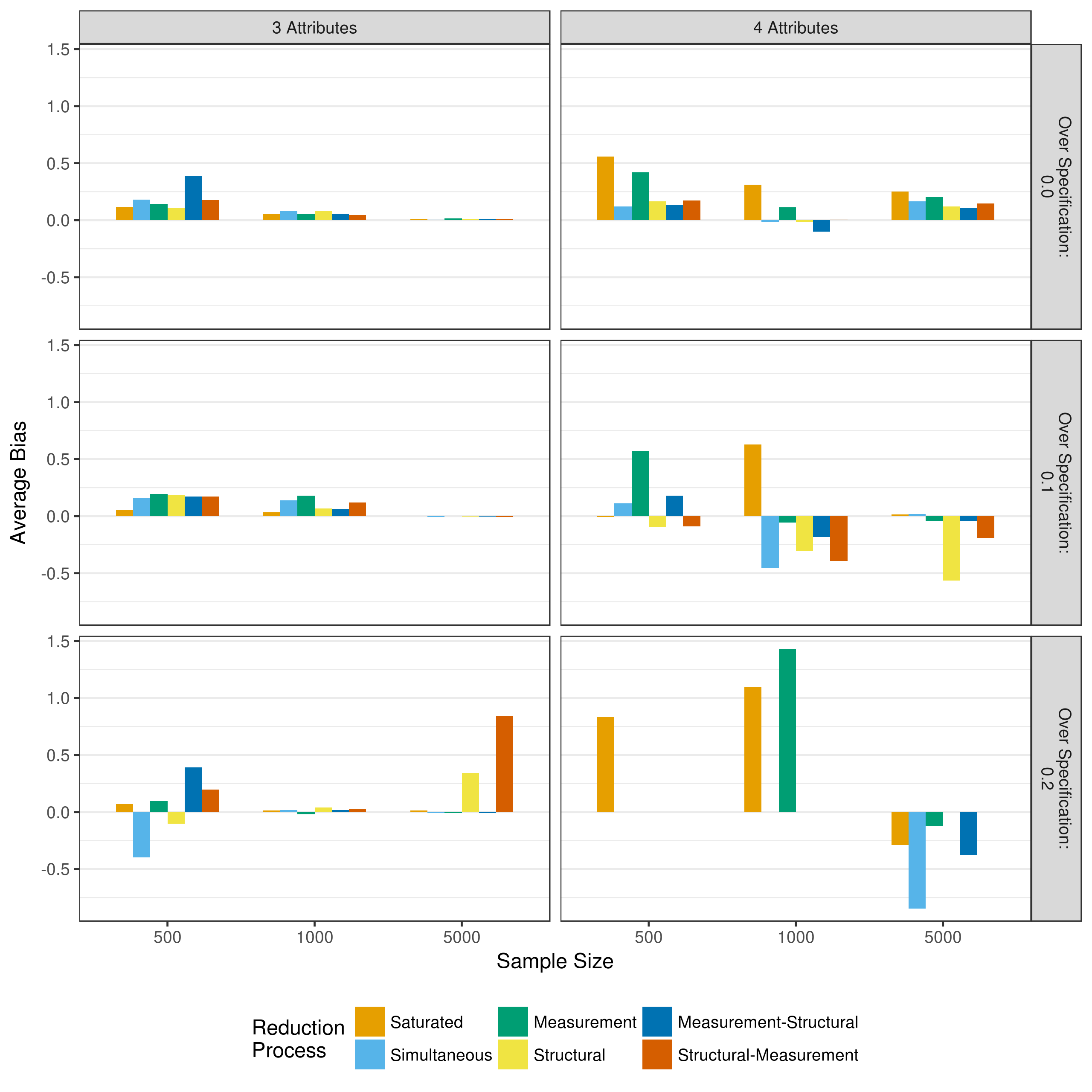
Figure 5.4: Bias in structrual model parameter estimates when reducing using p-values
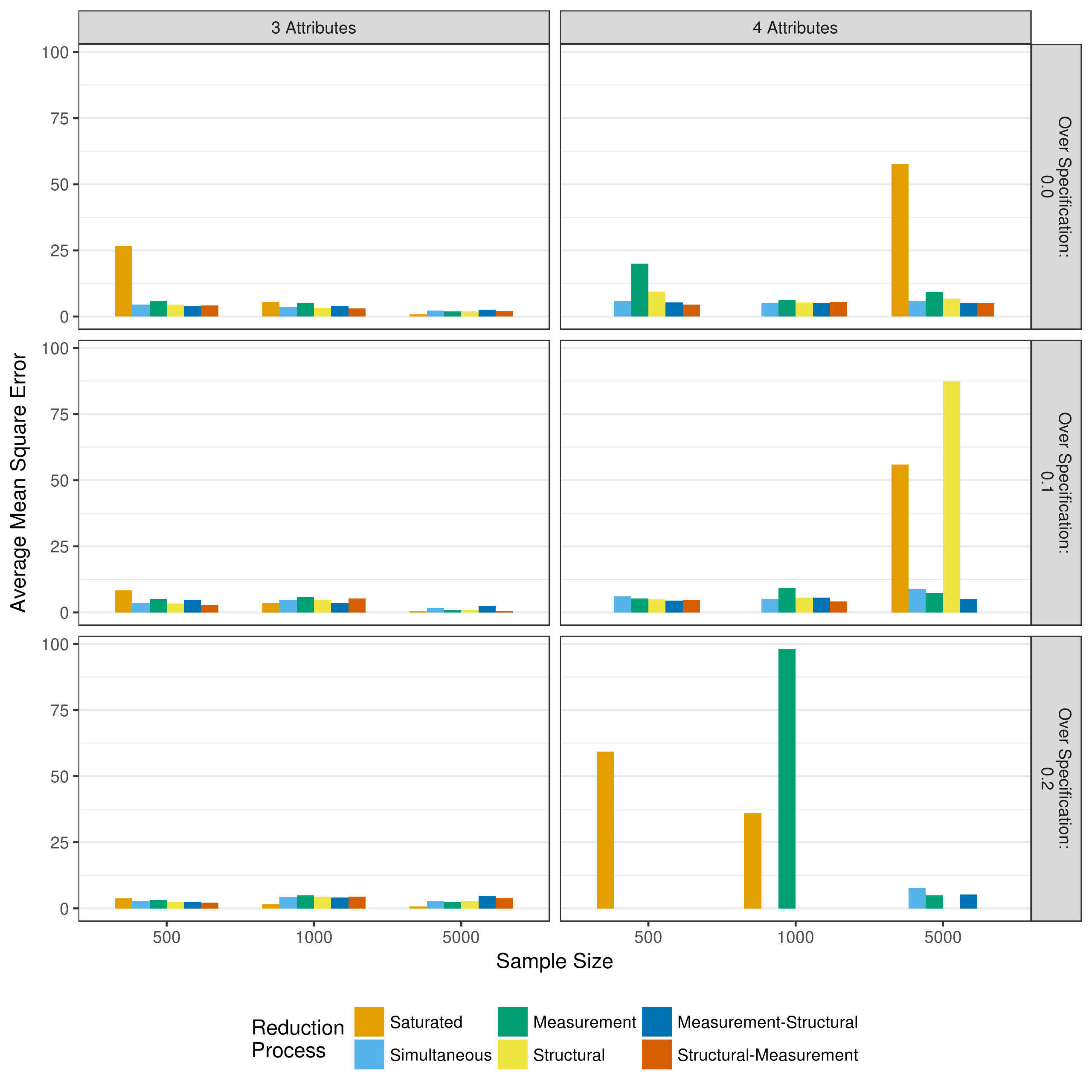
Figure 5.5: Mean square error in structrual model parameter estimates when reducing using p-values
5.1.3 Mastery classification
Another critical measure of performance is the rate at which respondents are correctly classified as masters of the attributes. This is assessed at two levels: the individual attribute classifications, and the overall profile classification. As described in section 4.2.4, profile mastery and attribute mastery differentiate between two types of assignments that can occur. For example, a respondent may have a true profile of [1,0,1,0] and an estimated profile of [1,1,1,0]. Here, the overall profile assignment is incorrect (profile classification), but three out of the four individual attributes are correctly classified (attribute classification). Respondents were classified as a master of an attribute if their posterior probability of mastery was greater than or equal to .5, and non-master of the attribute otherwise. Figure 5.6 and Figure 5.7 show the attribute level agreement as measured by the average correct classification rate and average Cohen’s \(\kappa\), respectively.
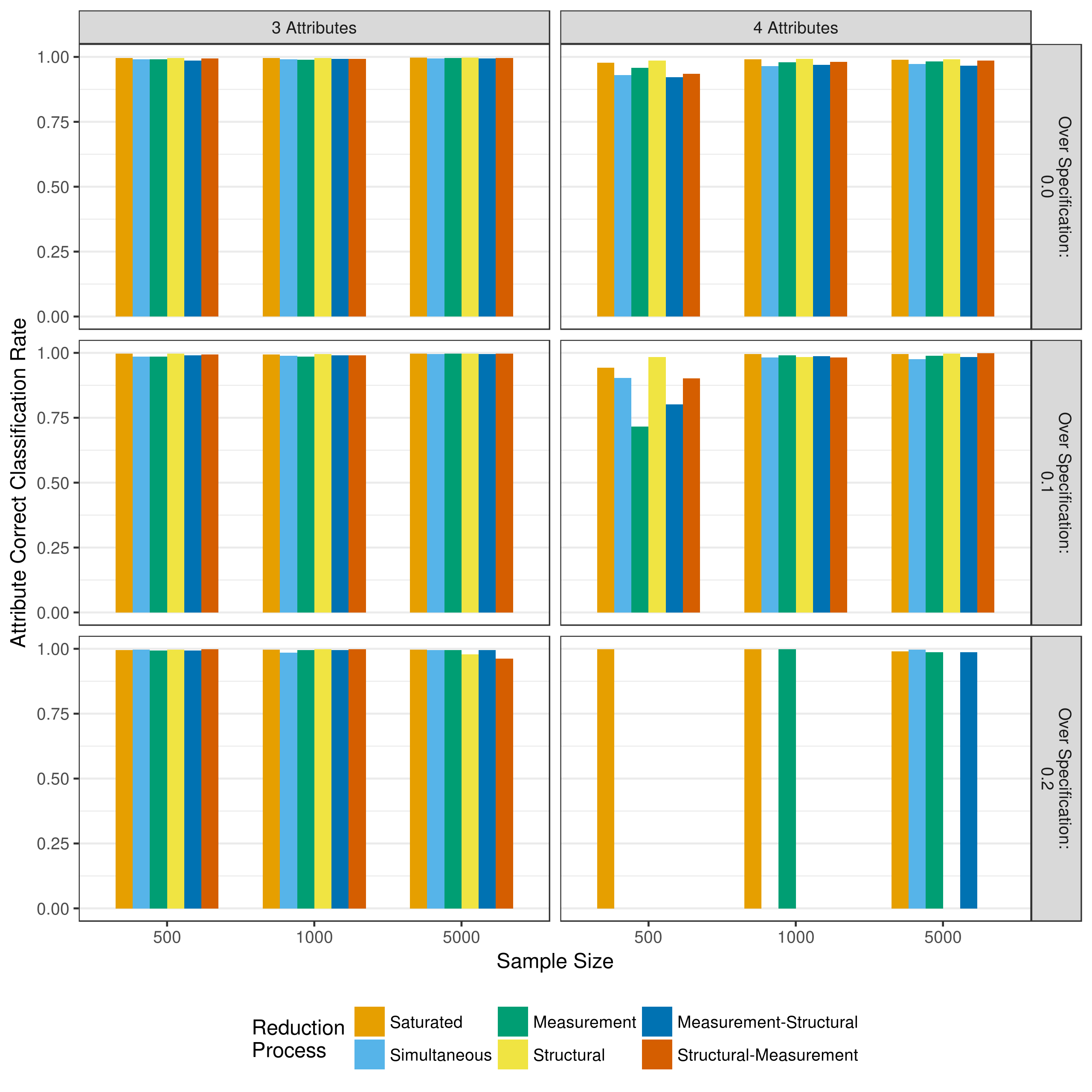
Figure 5.6: Average correct classification rate of attribute mastery when reducing using p-values
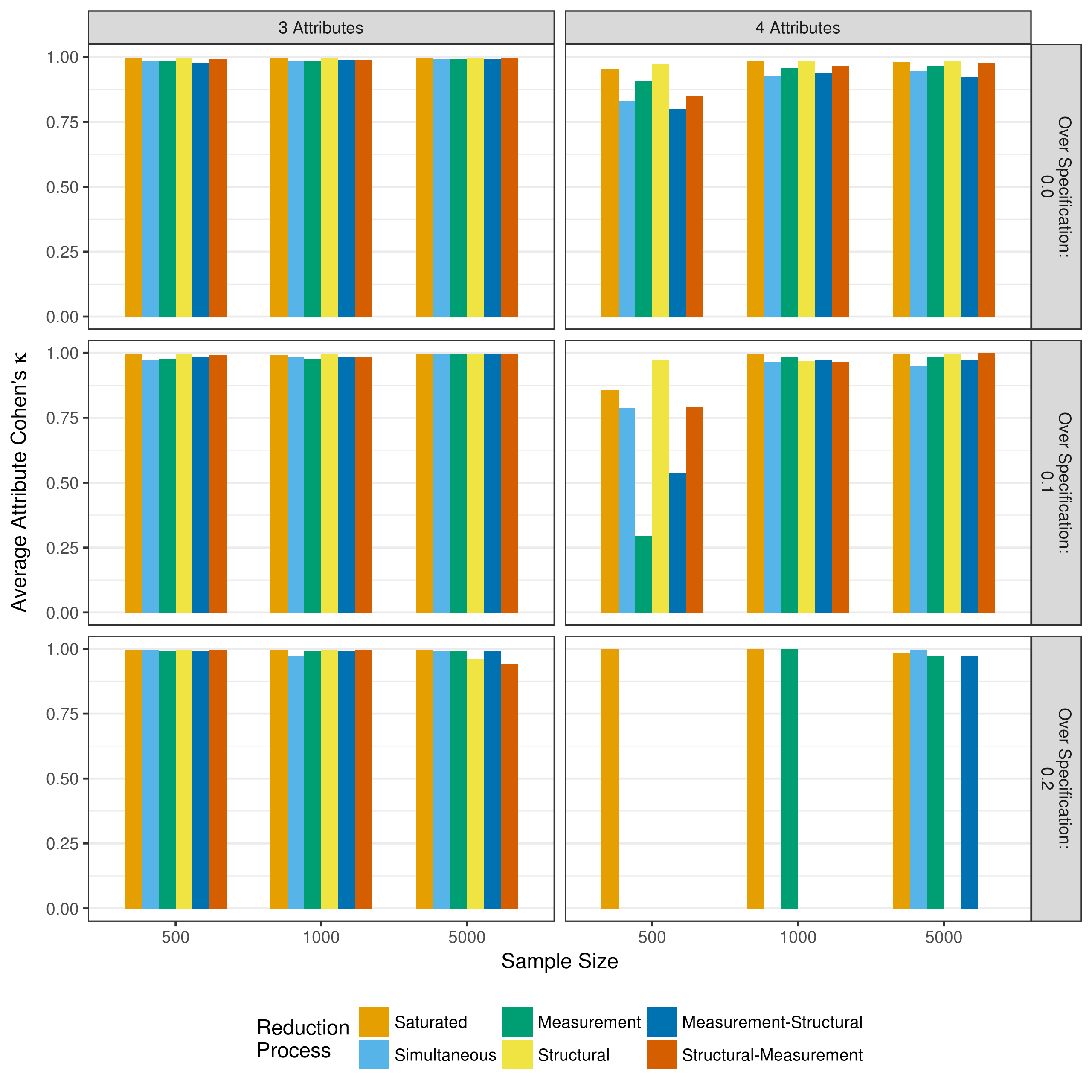
Figure 5.7: Average Cohen’s \(\kappa\) of attribute mastery when reducing using p-values
Across all conditions, both the correct classification rate and Cohen’s \(\kappa\) show high rates of agreement between true and estimated attribute classifications. The exception is a four-attribute assessment with a sample size of only 500. Under these conditions, all model reduction processes showed lower rates of agreement than with larger samples or only three attributes.
The overall profile classification shows a similar pattern. Figure 5.8 and Figure 5.9 show the correct classification rate and Cohen’s \(\kappa\) of the overall profiles. As expected, the overall profile agreement is consistently lower than the attribute level mastery classification agreement, although the classification agreement is generally consistent across all model reduction processes. Additionally, as with the attribute classifications, profile classification agreement was lower in the four-attribute, 500 sample size conditions.
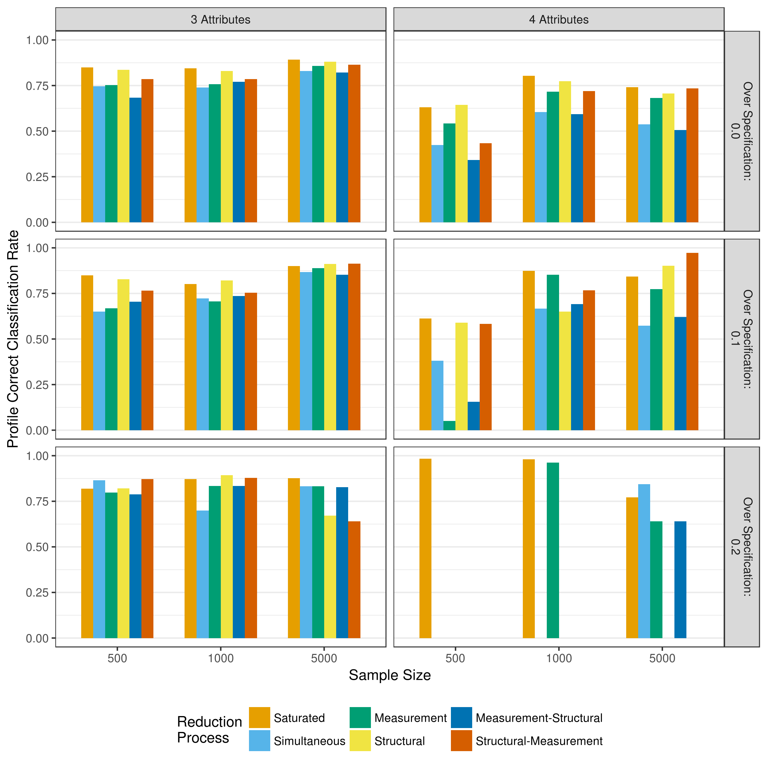
Figure 5.8: Average correct classification rate of profile assignment when reducing using p-values
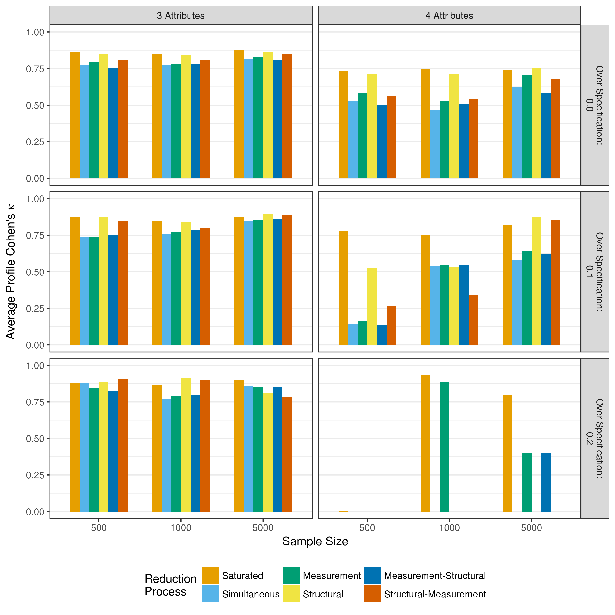
Figure 5.9: Average Cohen’s \(\kappa\) of profile assignment when reducing using p-values
5.1.4 Model fit
Critical to the model selection process is model fit. Although different model reduction processes may all show adequate recovery of item parameters and respondent classification, these measures cannot provide insight as to whether or not the removal of the parameters significantly impacted model fit. Figure 5.10, Figure 5.11, and Figure 5.12 show how many times the AIC, BIC, and adjusted BIC, respectively, selected each model reduction as the preferred model for a given data set.
Figure 5.10 shows a strong preference for the saturated model when using the AIC to pick the preferred model. This indicates that the additional parameters in the saturated model provide enough improvement to model fit to justify the additional complexity. However, structural reduction was also selected fairly often, especially in the true Q-matrix conditions. This suggests that the full structural model was often overly complex, and a reduced version provied adequate fit.
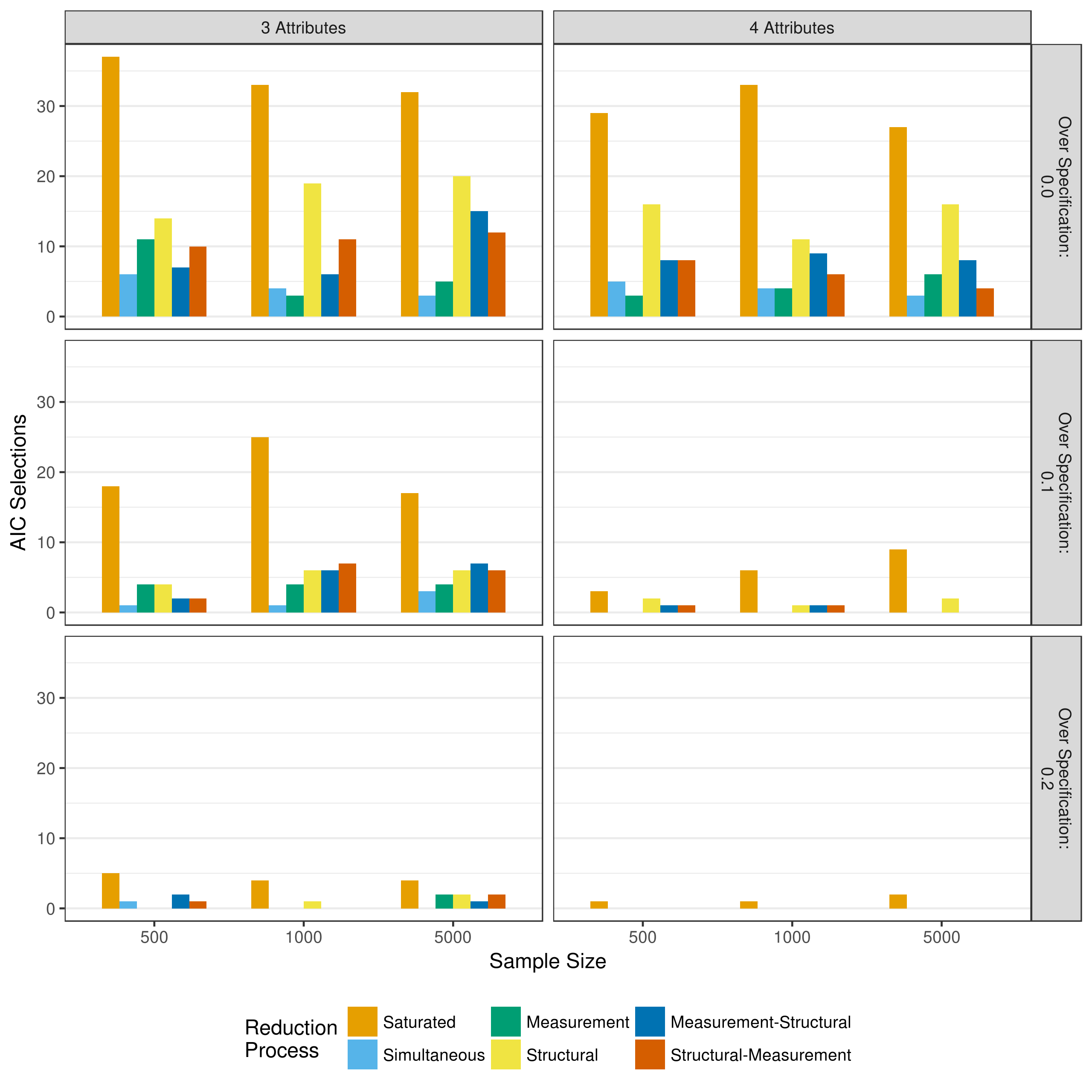
Figure 5.10: Number of selections as best fitting model as measured by the AIC when reducing using p-values
The BIC shows very different results (Figure 5.11). When selecting a model based on the BIC, the preferred method was most commonly structural-measurement, followed by measurement-structural reduction. This may be unsurprising, as the penalty for additional parameters is greater in the BIC than the AIC (Wit, van den Heuvel, & Romeijn, 2012). Therefore, the BIC is more likely to prefer models with fewer parameters. However, when the Q-matrix is correctly specified, the preference for the saturated model increases as the sample size increases. This indicates that model reduction may be more important when sample sizes are smaller, and it is more difficult to get good parameter estimates.
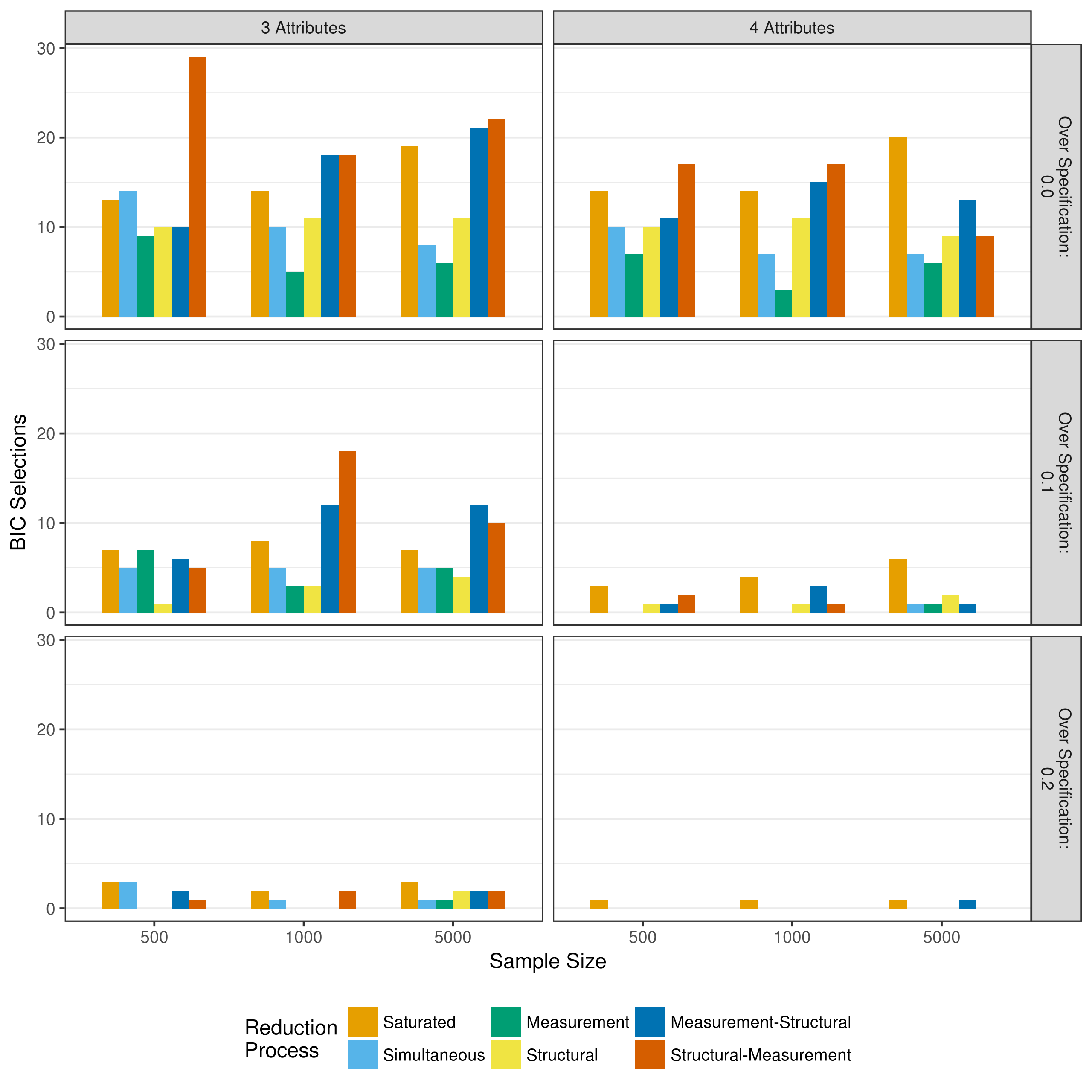
Figure 5.11: Number of selections as best fitting model as measured by the BIC when reducing using p-values
Finally, results when using the adjusted BIC show a middle ground between the results when using the AIC or BIC (Figure 5.12). There is still a strong preference for the saturated model, however, there is also a stronger preference for the structural-measurement and measurement-structural reductions than what was seen when using the AIC.
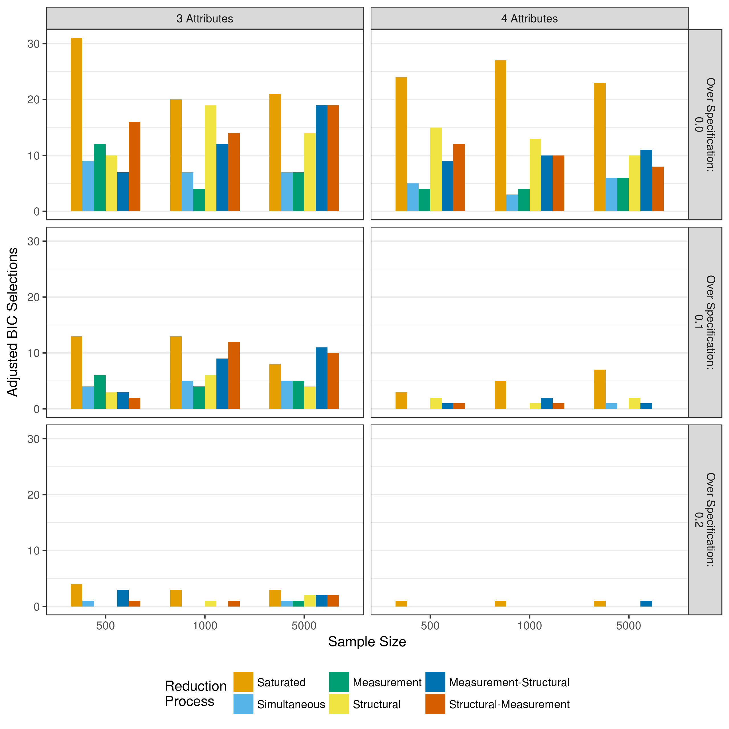
Figure 5.12: Number of selections as best fitting model as measured by the adjusted BIC when reducing using p-values
5.1.5 Description of reduced parameters
Another outcome of interest beyond the recovery of the generated parameters is how often each reduction process resulted in the correct parameters being included in the final model. For example, if an item measured only one attribute, but the Q-matrix specified two attributes, were the additional main effect and interaction term correctly removed? Conversely, if an item did in fact measure two attributes, were both main effects and the interaction term correctly retained? Figure 5.13 shows the proportion of time the measurement model was correctly reduced, and Figure 5.14 shows the proportion of correct reductions for the structural model.
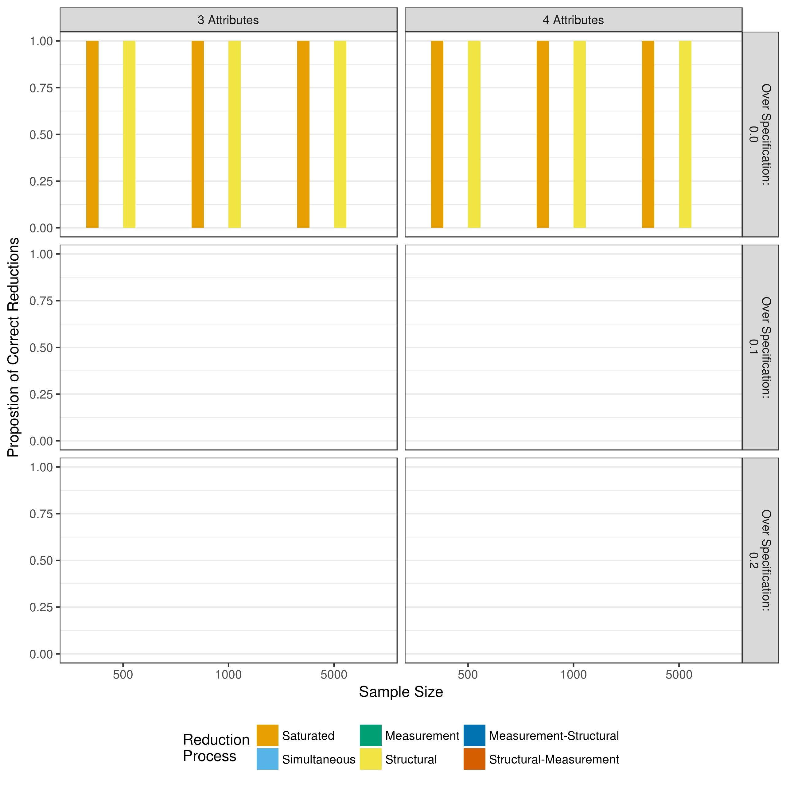
Figure 5.13: Proportion of correct measurement model reductions when reducing with p-values
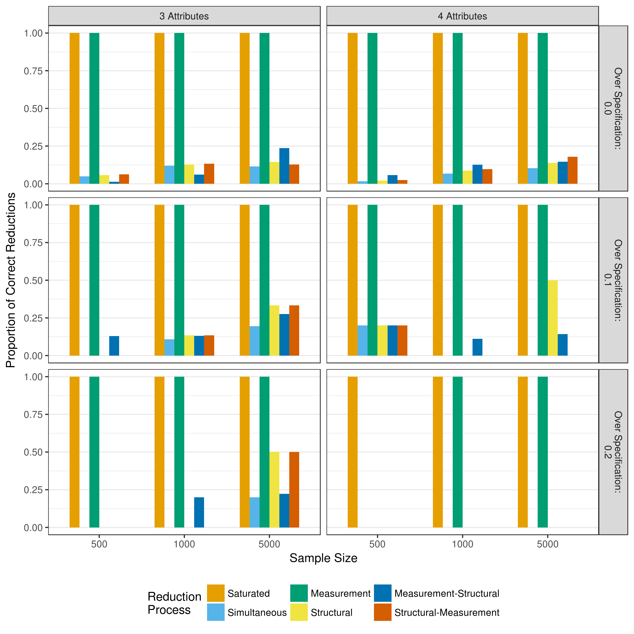
Figure 5.14: Proportion of correct structural model reductions when reducing with p-values
Figure 5.13 shows that the only cases where the correct measurement model was obtained was when it was correctly specified, and no parameters were removed (i.e., saturated model or only structural reduction). These results should be interpreted with caution. A “correct” measurement model is defined as all parameters in the final model exactly matching the parameters used to generate the data. This does not account, however, for parameters that may have contributed to the data generation, but not in a significant way. For example, the main effects were drawn from a uniform distribution (0.00, 5.00]. Thus, it is entirely plausible, and expected, for main effects with a value close to zero to be drawn. Thus, these parameters would technically be part of the true measurement model, but may not be statistically significant, and even one of these parameters would result in the determination of an incorrect measurement model.
A similar pattern is seen in Figure 5.14, with very low rates of correct reduction, except when no reduction of the structural model was performed (i.e., saturated model or only measurement reduction). Because the data was always generated with a fully saturated log-linear structural model, and reduction of the structural model results in a determination of an incorrect reduction. However, given that the structural parameters were all drawn from a \(\mathcal{N}(0, 2)\) distribution the same caveats of significance apply that applied to the measurement model parameters.
To verify that the parameters being reduced are indeed these parameters that are very small, and thus may not be significant, the distributions of estimates and standard errors of the reduced parameters can be examined. Figure 5.15 shows that the majority of reduced measurement model parameters are small in value, with small standard errors. More parameters were removed from the true Q-matrix conditions than the over specified Q-matrix conditions, however this is an artifact of the over specified conditions converging far less often.
Figure 5.16 shows a similar pattern for the structural parameters, with the majority of reduced parameters having an estimate close to zero. Additionally, the most of the reduction occurred out of the true Q-matrix conditions, as the over specification conditions often failed to converge. However, unlike the measurement model parameters, there is more variability in the estimates and standard errors of the parameters that were reduced.
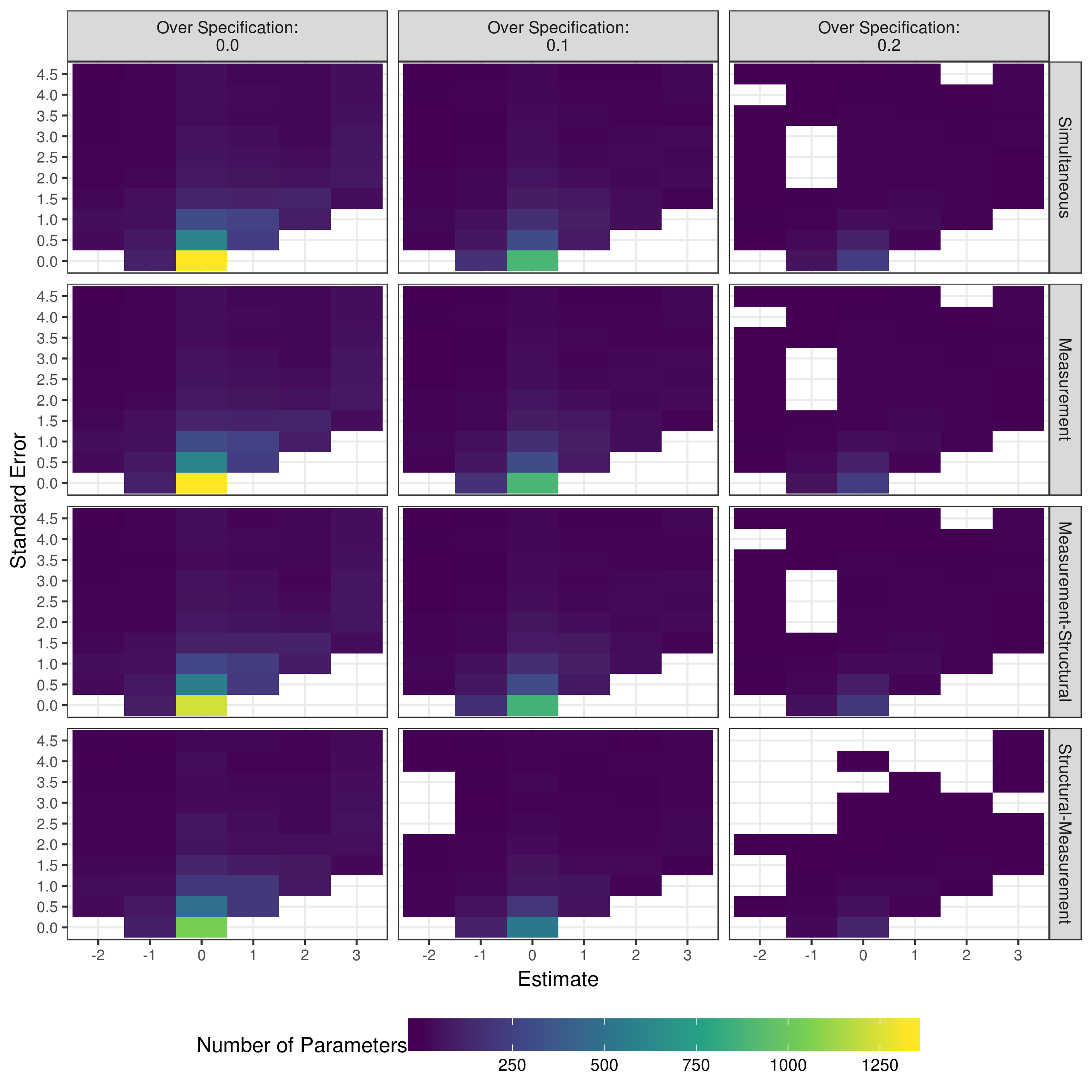
Figure 5.15: Distributions of estimates and standard errors for reduced measurement model parameters when reducing with p-values
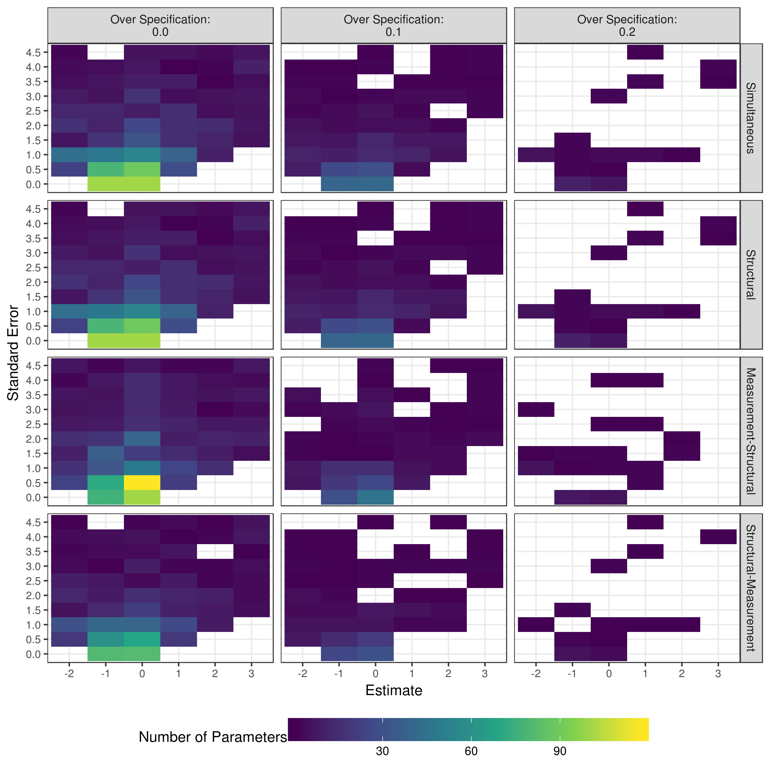
Figure 5.16: Distributions of estimates and standard errors for reduced structural model parameters when reducing with p-values
5.2 Reduction by heuristic
When the saturated model failed to converge, high level interaction parameters (i.e., three- and four-way interactions) were selected for reduction from the measurement and structural models. Following this initial heuristic reduction, if the model converged, the reduction processes continued using p-values (Figure 4.1). Whereas section 5.1 described the performance of model that were reduced using p-values at all steps of model reduction, this section describes the second scenario, where models were reduced with the heuristic first, and then p-values.
5.2.1 Convergence
Figure 5.17 shows the convergence rates for these reduction processes when the saturated model failed to converge. Recall that measurement-structural and structural measurement reduction only occurred if the measurement and structural reductions using the heuristic, respectively, converged. When the Q-matrix is correctly specified, reduction of the structural model led to convergence the majority of the time. Conversely, the removal of three- and four-way interactions in the measurement model never led to convergence, unless the structural was being reduced simultaneously. The measurement model was able to be reduced by p-values, but only after higher order interactions had been reduced from the structural model.
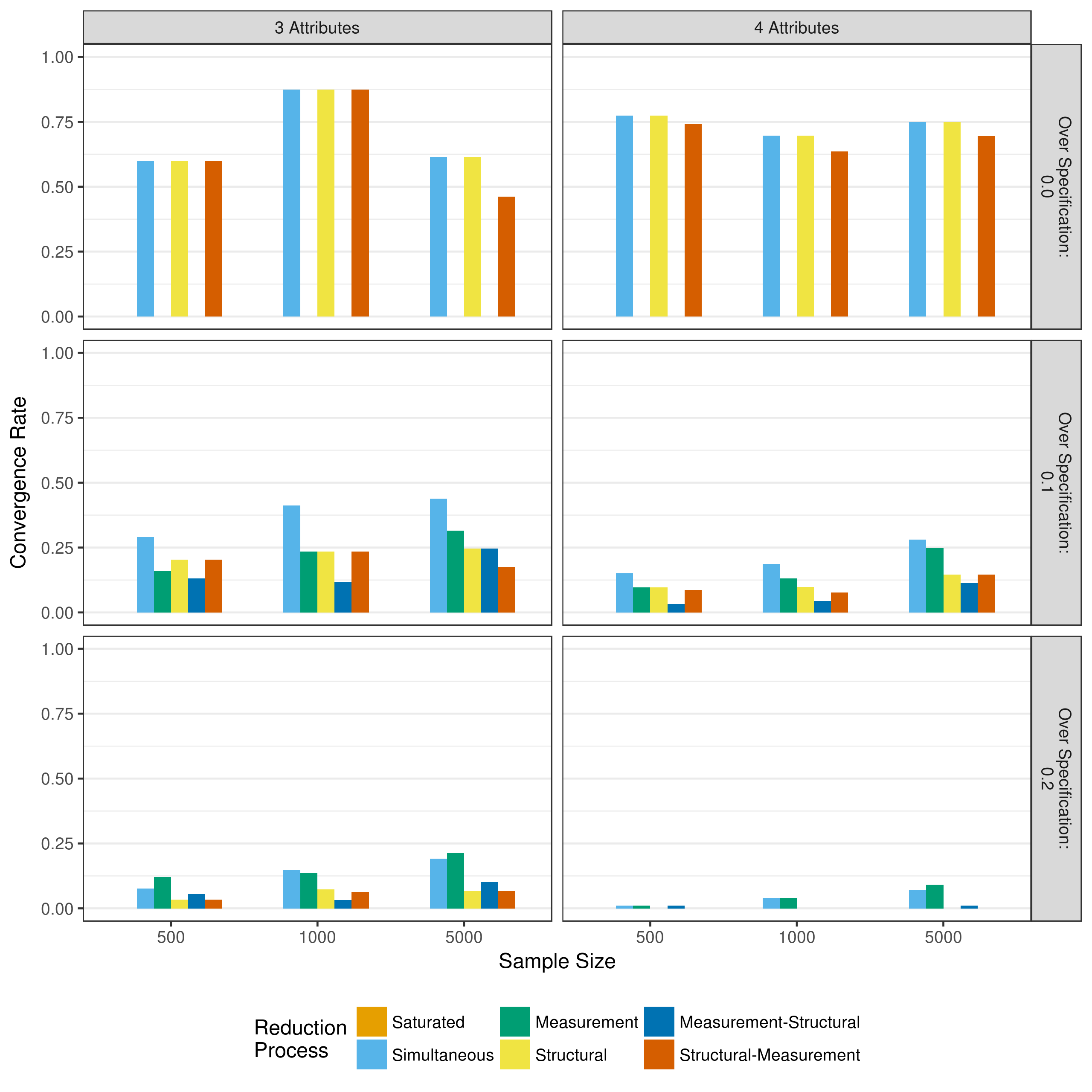
Figure 5.17: Convergence rates when reducing using a heuristic
In contrast to the truly specified Q-matrix conditions, models rarely converged when the Q-matrix was over specified, regardless of reduction process. This was especially true as the complexity and amount of over specification increased. However, across these conditions, simultaneous reductions and measurement model reduction had the most success in getting the model to converge.
5.2.2 Parameter recovery
As with the reduction process that relied entirely on p-values, the bias and mean square error of the parameter estimates can be examined for models that used the heuristic as the first reduction step. Figure 5.18 and Figure 5.19 show the total bias and total mean square error, respectively, across all measurement model parameters when reducing using p-values. As with the Because of some outlying data sets, biases with an absolute value greater than 100 and mean square errors with a value greater than 100 have been excluded from the figures. Figures showing all biases and mean square errors, separated by the type of parameter can be seen in Appendix B.
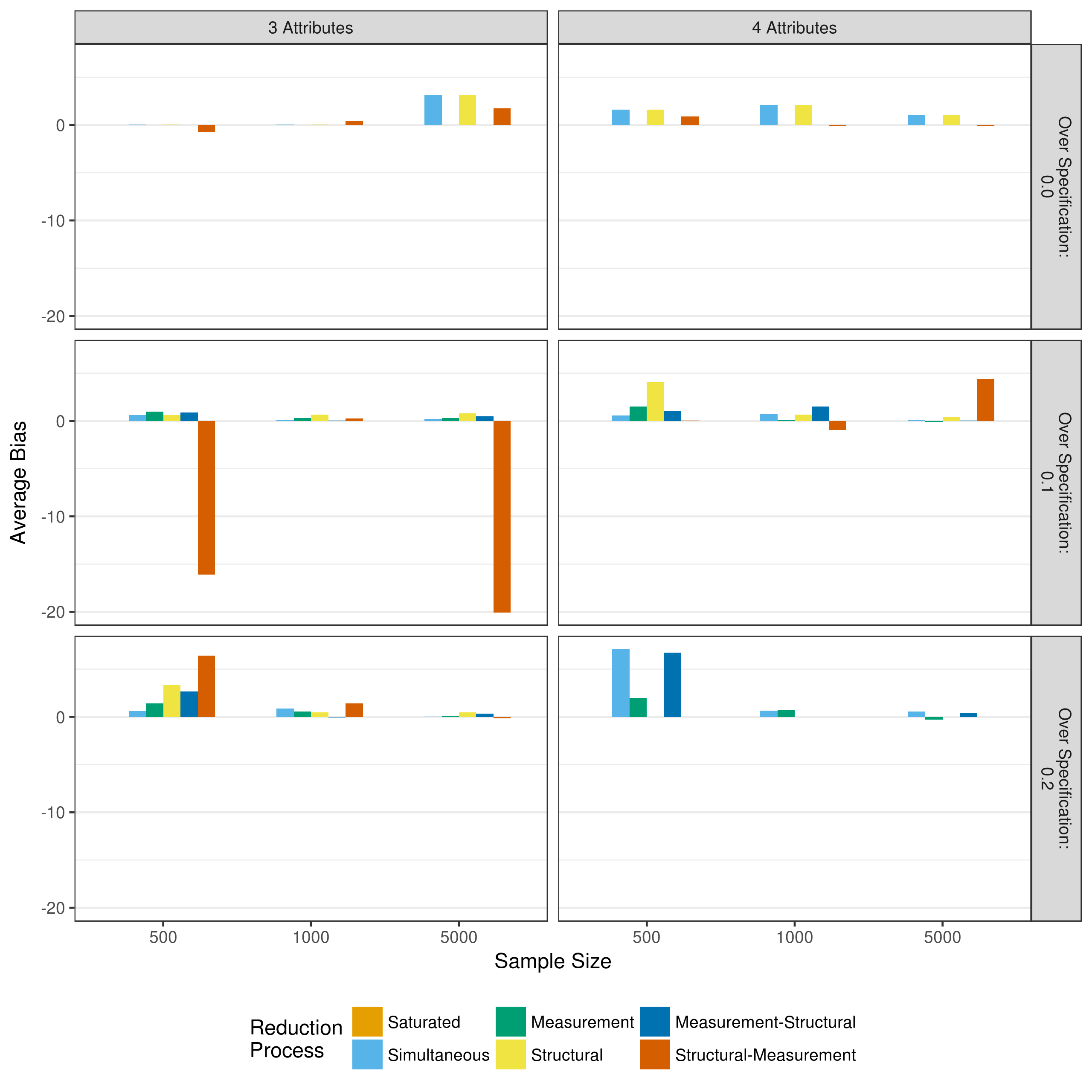
Figure 5.18: Bias in measurement model main effect estimates when reducing using a heuristic
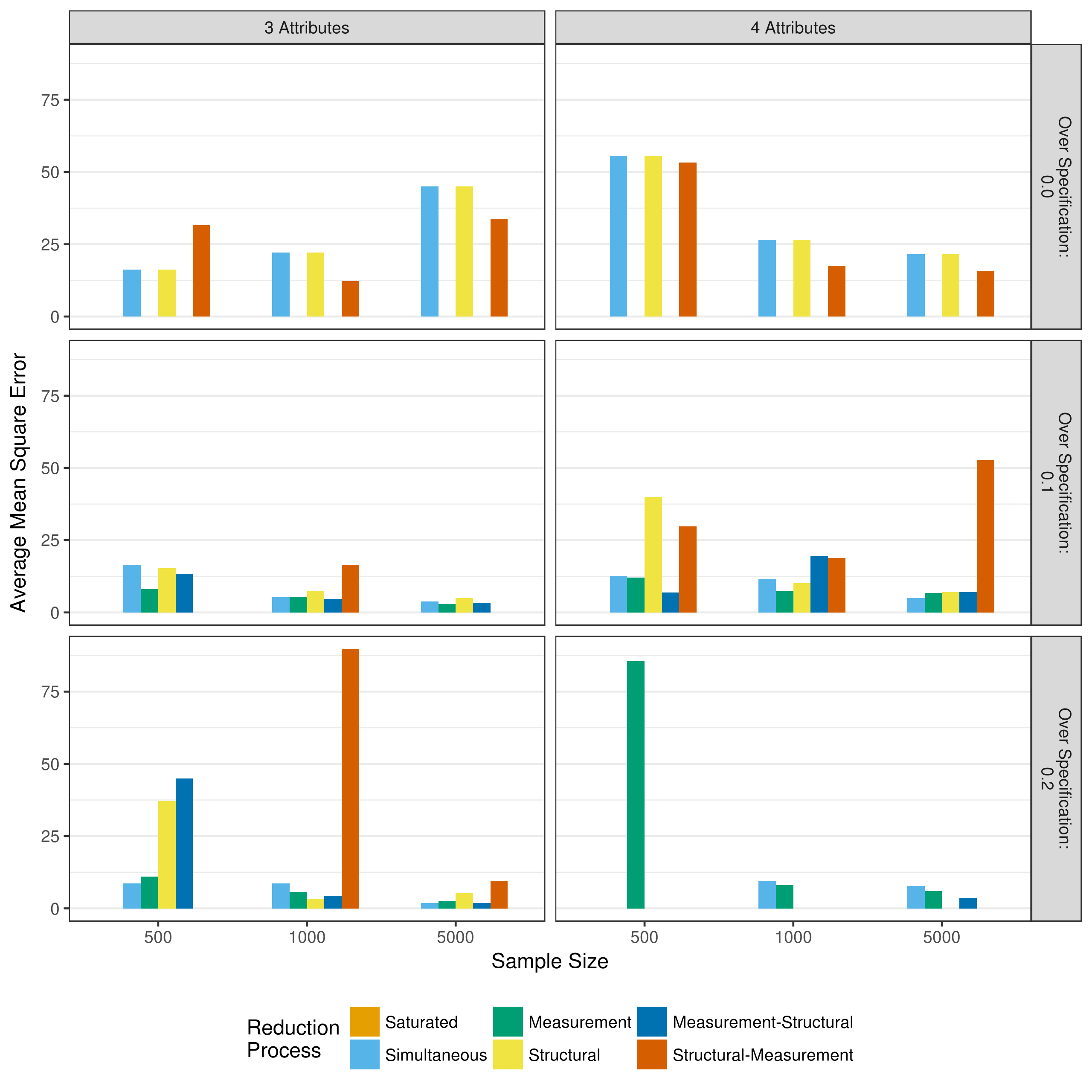
Figure 5.19: Mean square error in measurement model main effect estimates when reducing using a heuristic
Figure 5.18 shows that across all conditions, as with p-value based reduction, there is relatively little bias in the measurement model parameters, especially when the Q-matrix is correctly specified. The large negative biases seen in the structural-measurement reduction condition for the three attribute and 10 percent over specified Q-matrix are due to a couple of outlying data, as can be seen in Appendix B. Also similar to the reduction processes based entirely on p-values, there is relatively large mean square error values across conditions. As expected, and as with the p-value reduction, this decreases as the sample size increases.
Figure 5.20 and Figure 5.21 show the bias and mean square error of the structural parameters respectively. Overall, there is very little bias and mean squared error in the structural parameters. The instances where larger bias and mean squared error are indicated (e.g., 10 and 20 percent over specified Q-matrix) are instances where very few of the model actually converged. Thus, these values are based on only a few replications. Thus, these results suggests that, as with p-value only reduction, the structural parameters are usually well estimated regardless of model reduction method.
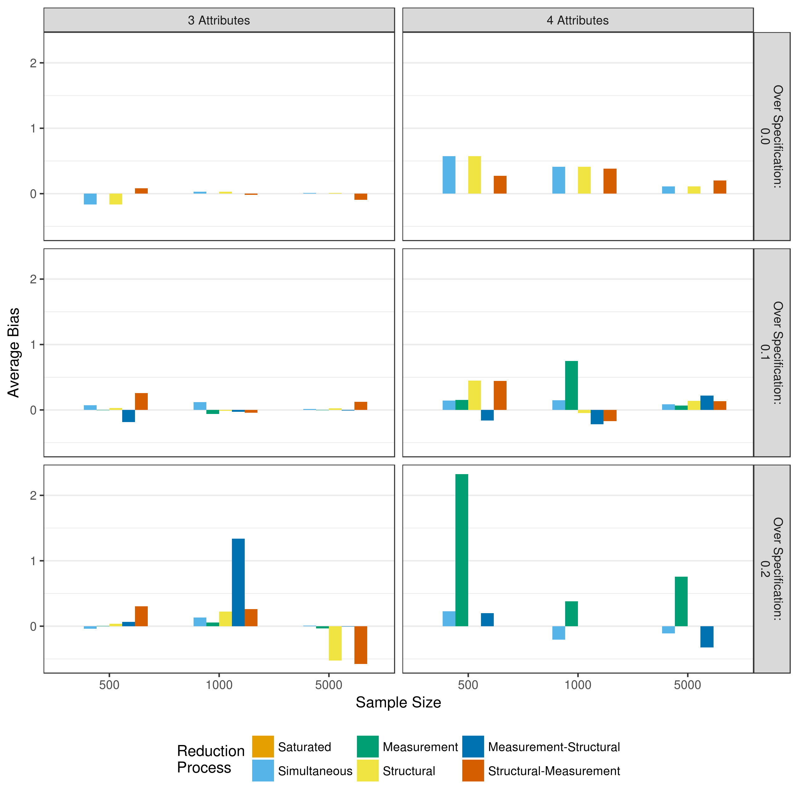
Figure 5.20: Bias in structrual model parameter estimates when reducing using a heuristic
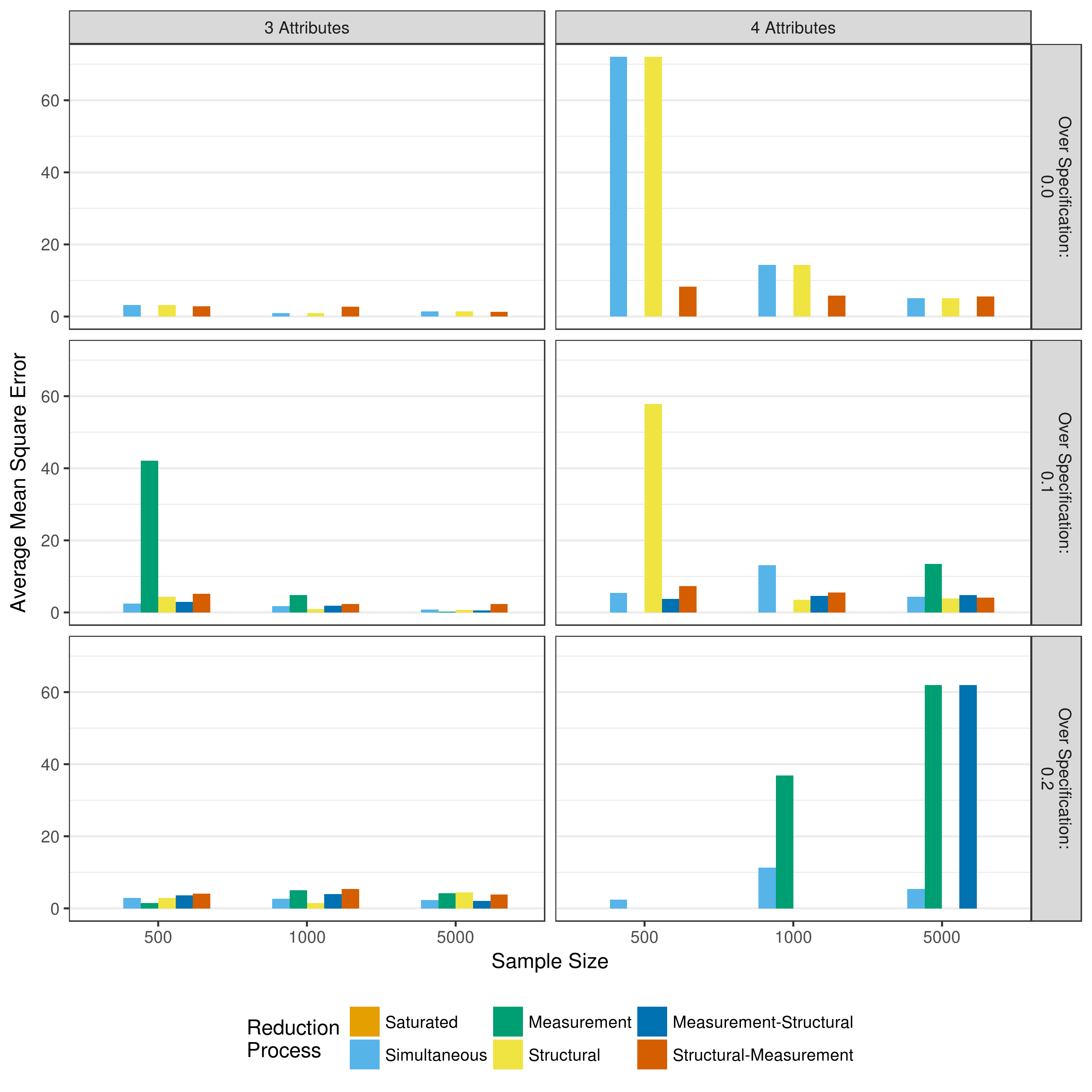
Figure 5.21: Mean square error in structrual model parameter estimates when reducing using a heuristic
5.2.3 Mastery classification
Just as with reduction based on p-values, it is important to evaluate mastery classification (at the attribute and profile level) when the initial reduction step is based on a heuristic. Figure 5.22 and Figure 5.23 show the attribute level agreement as measured by the average correct classification rate and average Cohen’s \(\kappa\), respectively.
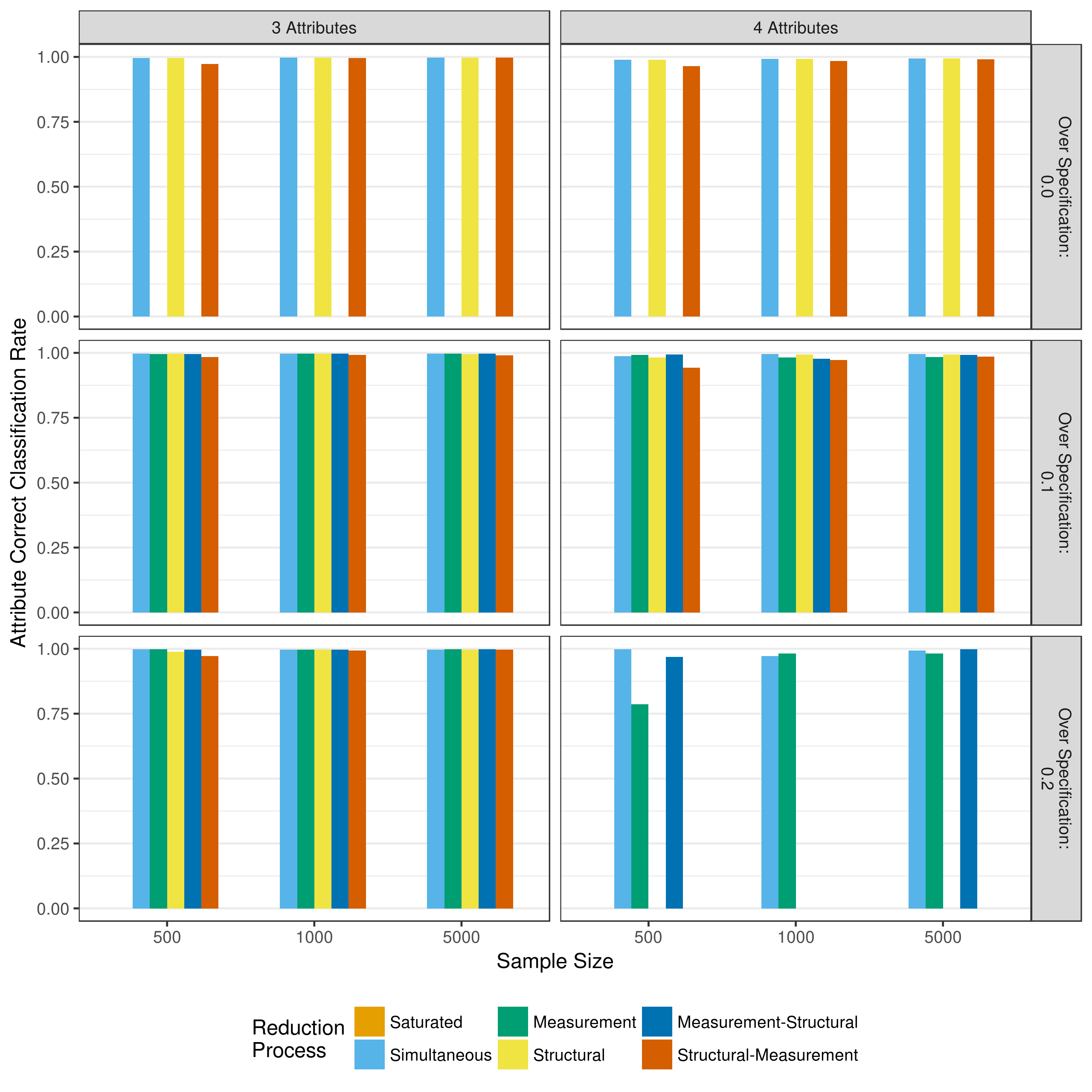
Figure 5.22: Average correct classification rate of attribute mastery when reducing using a heuristic
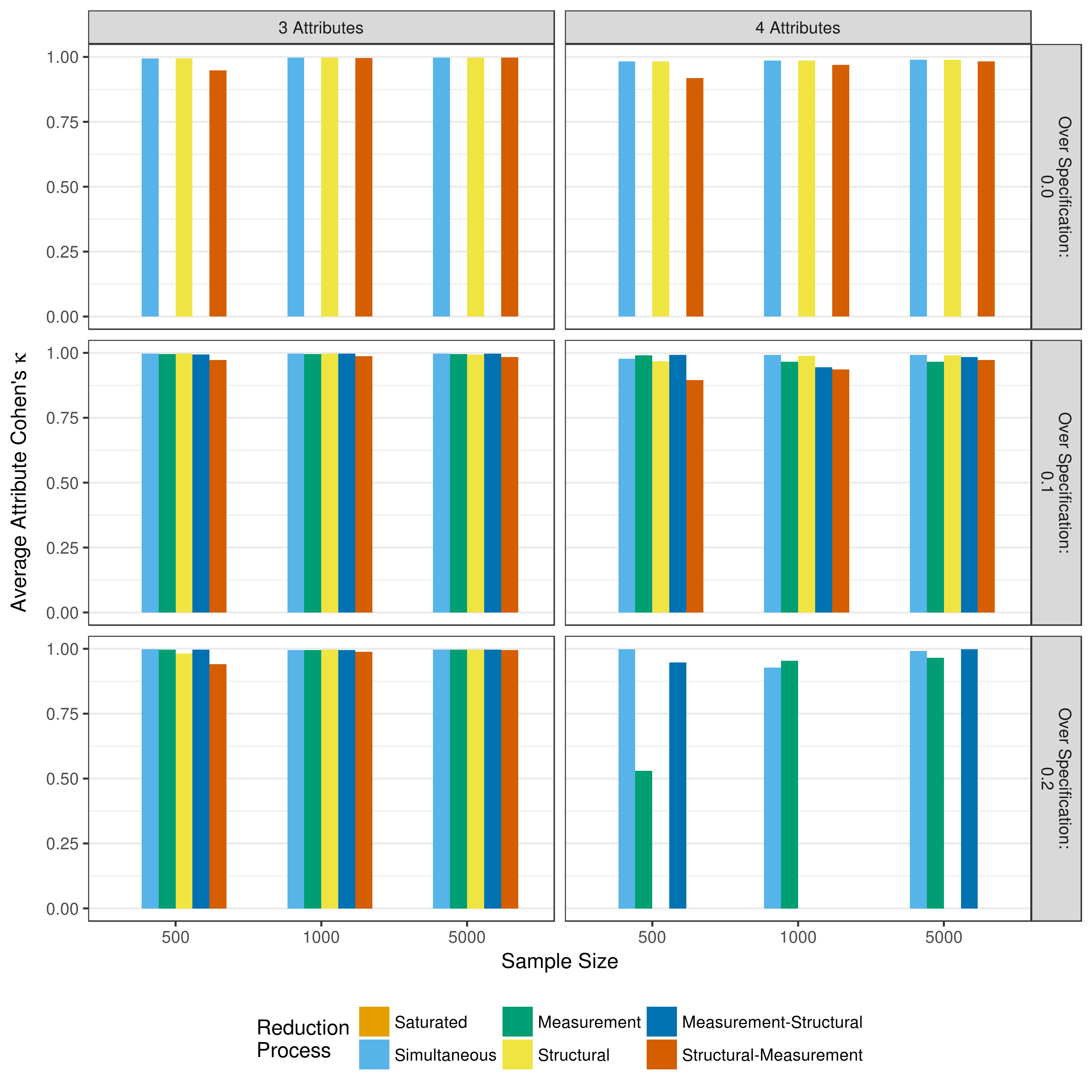
Figure 5.23: Average Cohen’s \(\kappa\) of attribute mastery when reducing using a heuristic
Across all conditions, both the correct classification rate and Cohen’s \(\kappa\) show high rates of agreement between true and estimated attribute classifications, just as was observed when using p-values for all reductions.
The overall profile classification shows also shows pattern similar to the p-value only reduction (Figure 5.24 and Figure 5.25). The overall profile agreement is consistently lower than the mastery classification at the attribute but, but the profile agreement is generally consistent across all model reduction processes.
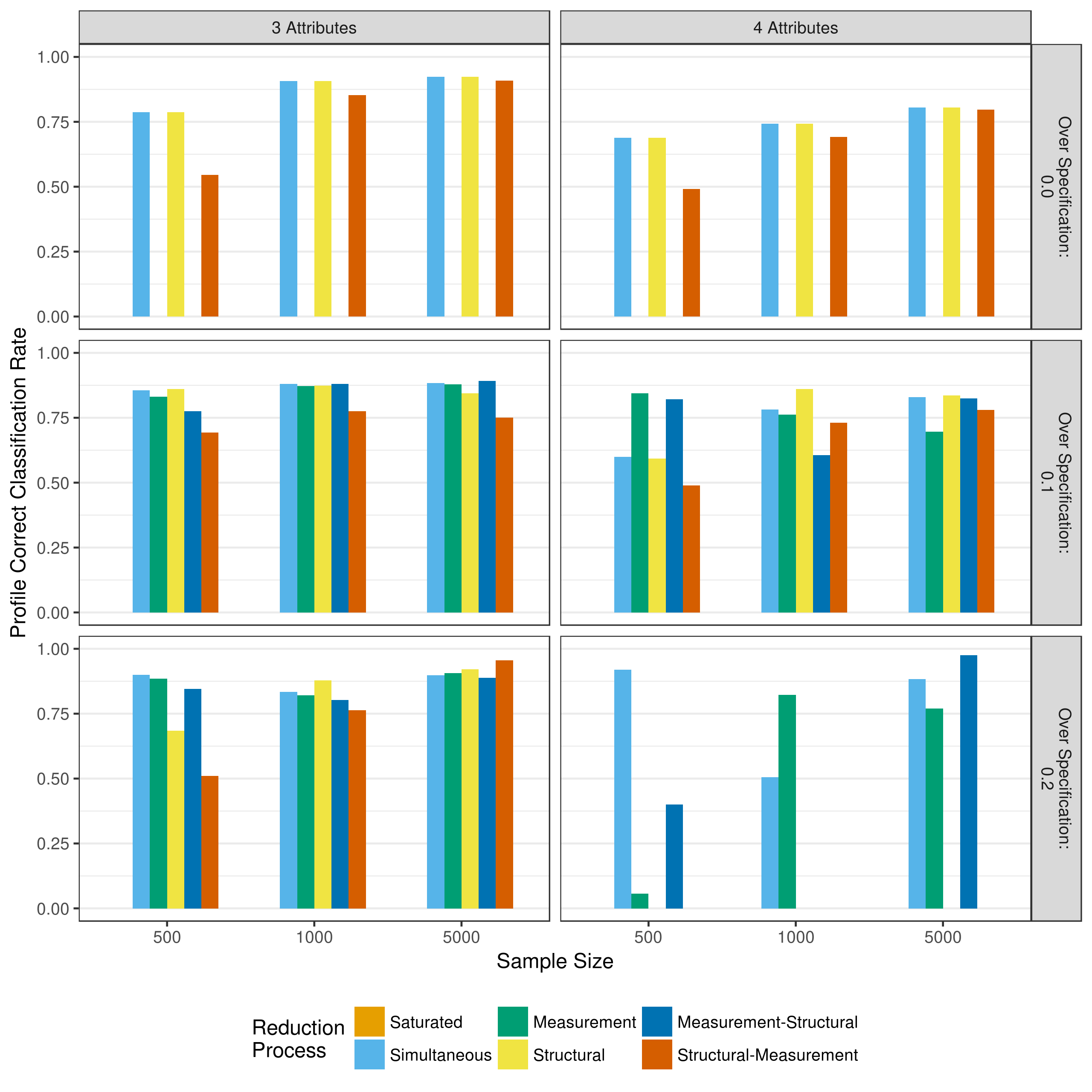
Figure 5.24: Average correct classification rate of profile assignment when reducing using a heuristic
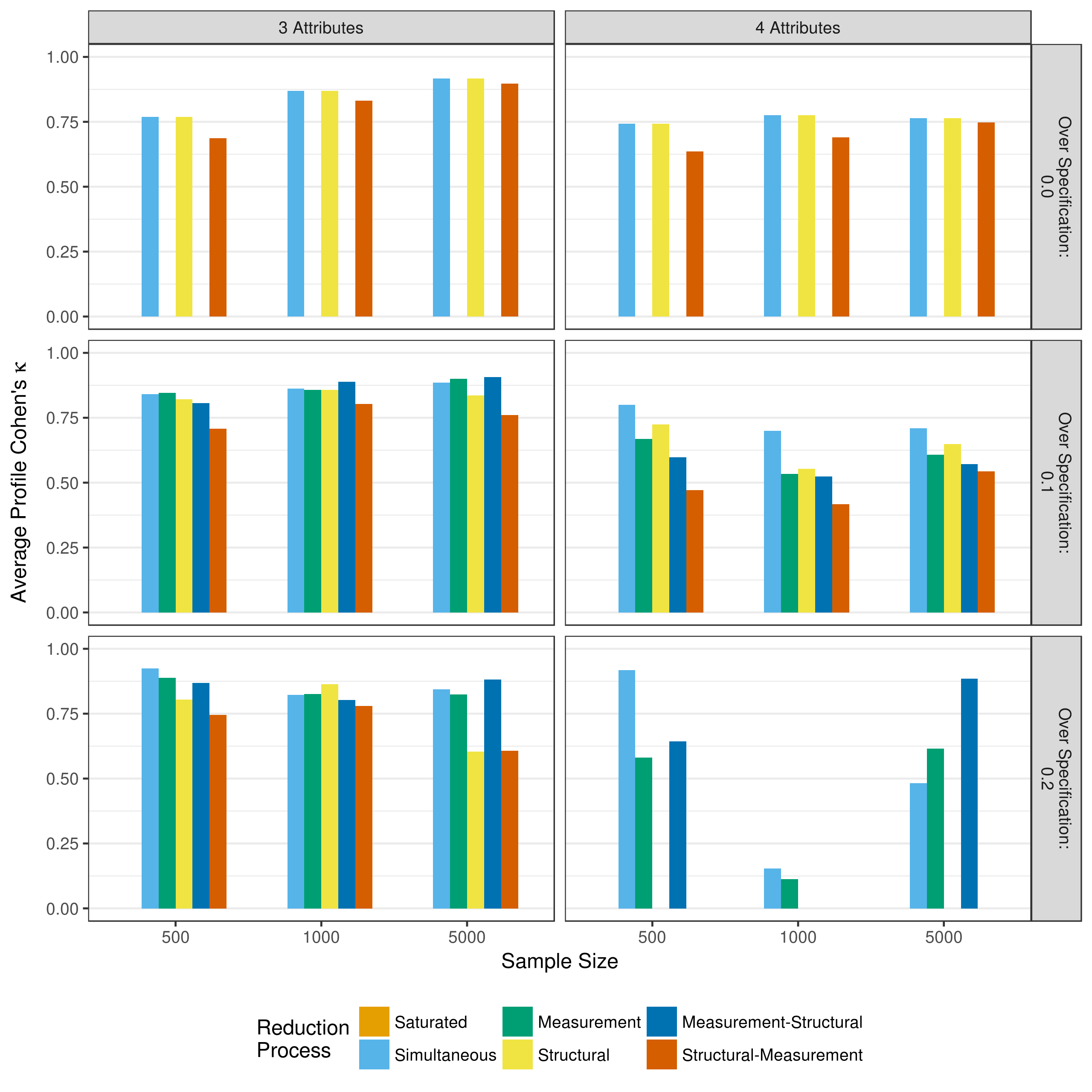
Figure 5.25: Average Cohen’s \(\kappa\) of profile assignment when reducing using a heuristic
5.2.4 Model fit
When the saturated model fails to converge and the model reduction process uses a heuristic to remove parameters, it is still important to assess model fit. Figure 5.26 shows the results when using the AIC to select the preferred model. When the Q-matrix is correclty specified, there is a strong preference for structural reduction over structural-measurement redcution. In contrast, when the Q-matrix is over specified, there is a stronger preference for simultaneous reduction of structural and measurement models. This preference is stronger as the amount of over specification increases.
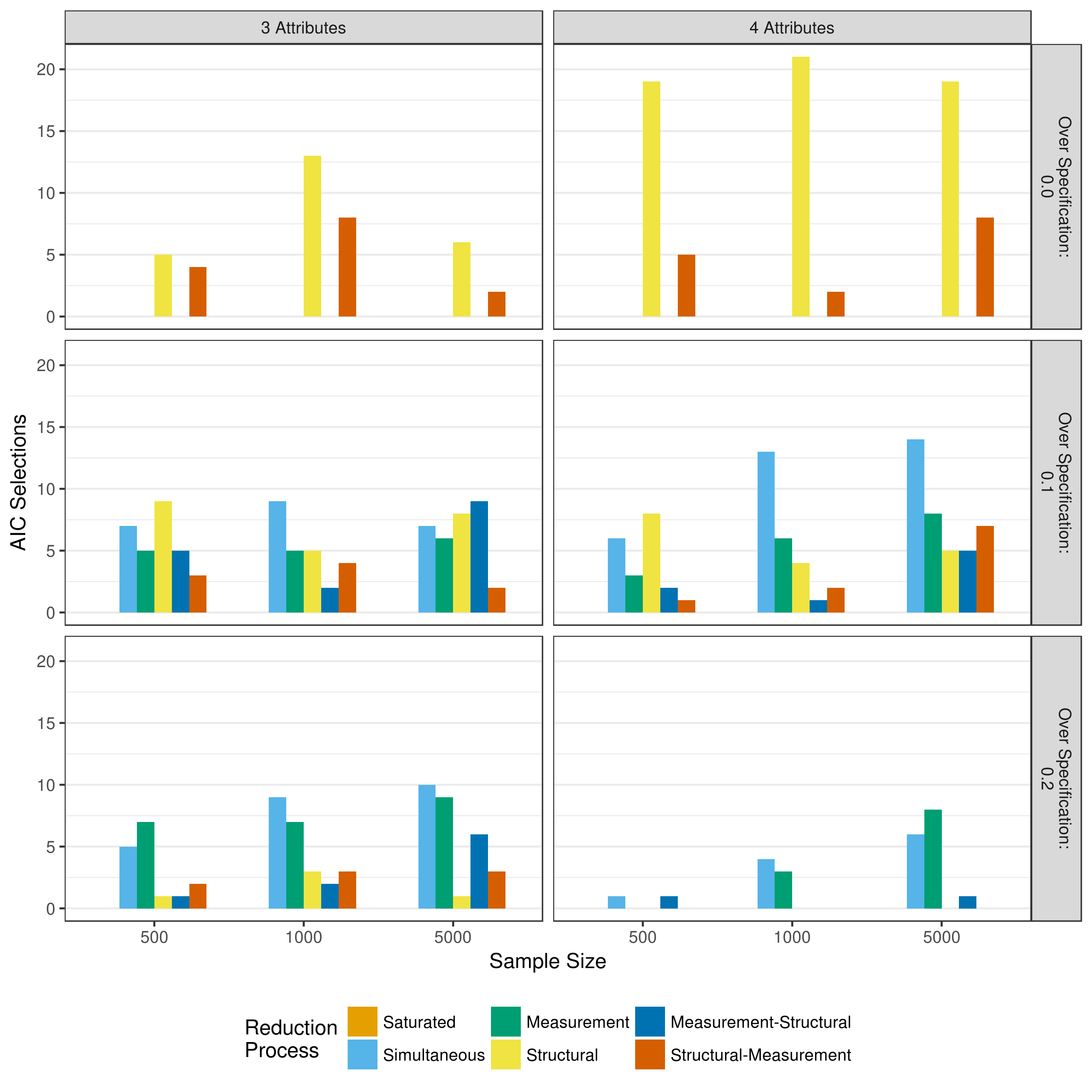
Figure 5.26: Number of selections as best fitting model as measured by the AIC when reducing using a heuristic
The BIC results in Figure 5.27 are similar to those seen when reduction depends only on p-values. There is a much stronger preference for structural-measurement and measurement-structural reduction than when using AIC. However, the difference is not as pronounced as with p-value only reduction, as simultaneous reduction is still preferred overall. Further, just as with the AIC, the preference for measurement reduction increases as the amount of over specification increases.
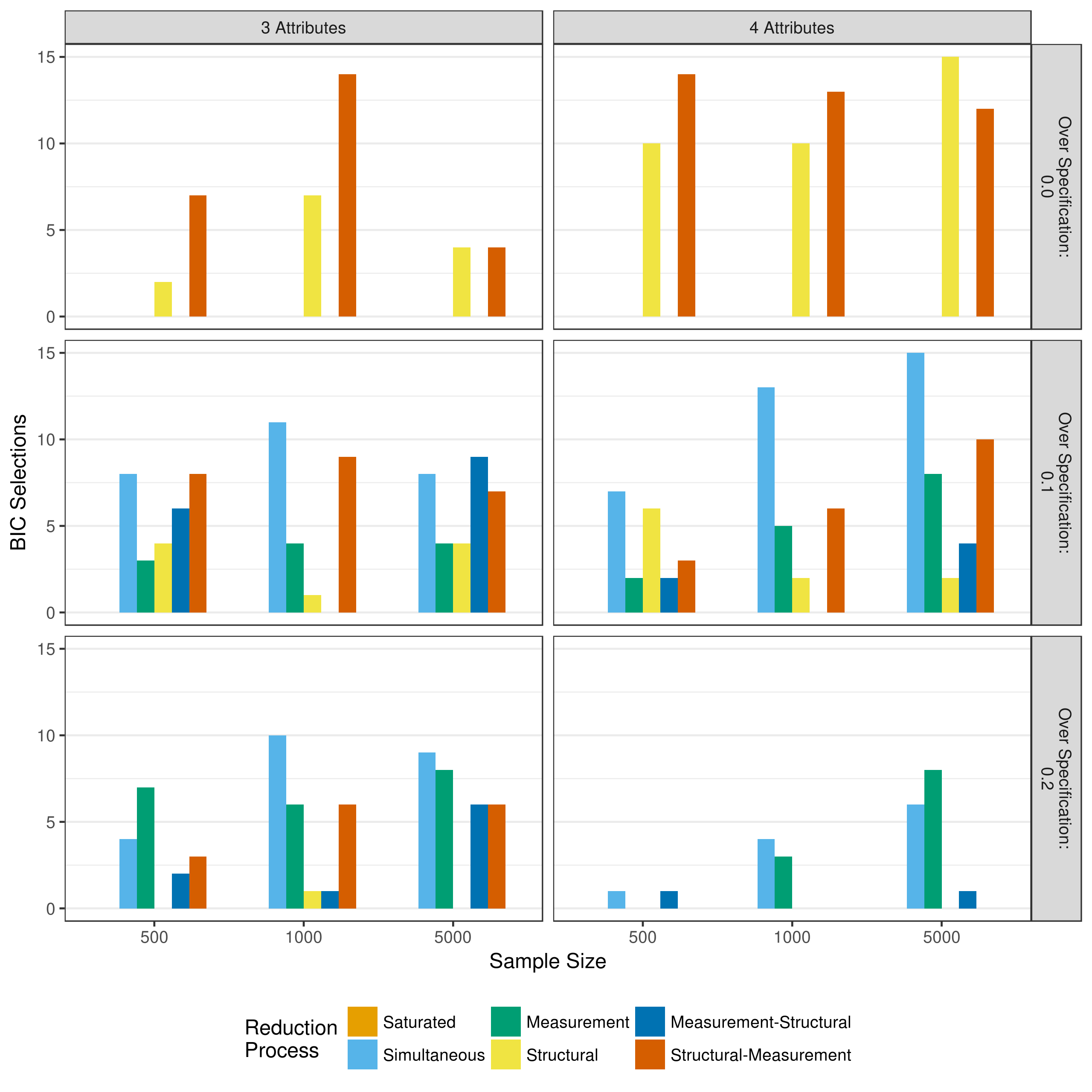
Figure 5.27: Number of selections as best fitting model as measured by the BIC when reducing using a heuristic
The model selection when using the adjusted BIC is also reflective of the results found when using only p-values (Figure 5.28). That is, the adjusted BIC serves as a middle ground between the AIC and the BIC. There is a stronger preference for the structural-measurement and measurement-structural reduction processes than when using the AIC, but not as strong when using the BIC. Additionally, there is a stronger preference for measurement model reduction as the amount of over specification in the Q-matrix increases.
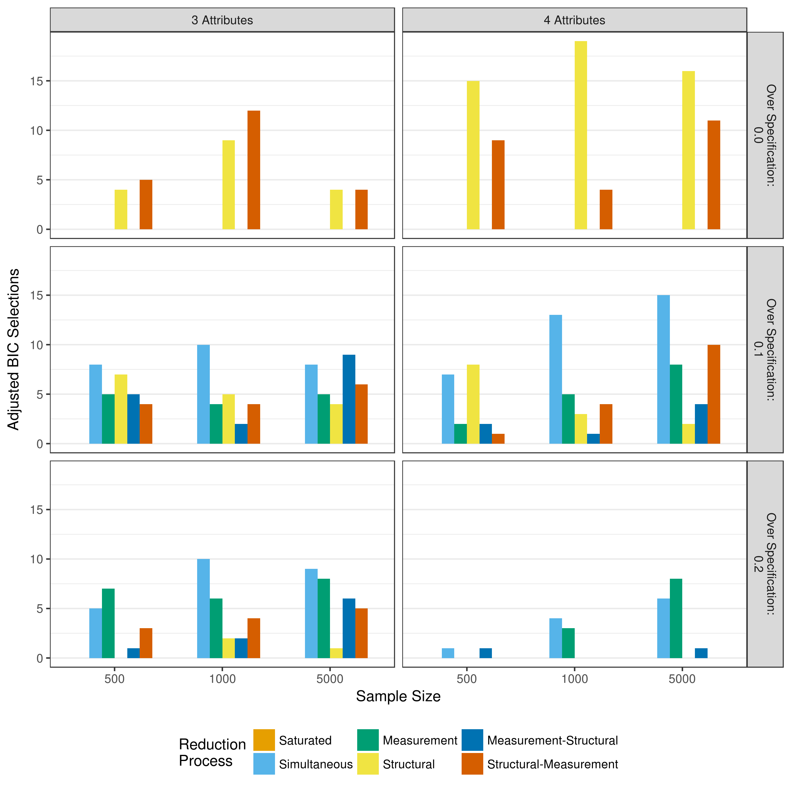
Figure 5.28: Number of selections as best fitting model as measured by the adjusted BIC when reducing using a heuristic
5.2.5 Description of reduced parameters
Finally, the performance of the different processes in terms of correctly specifying the parameters to be included can be examined. Figure 5.29 shows the proportion of time the measurement model was correctly reduced, and Figure 5.30 shows the proportion of correct reductions for the structural model.
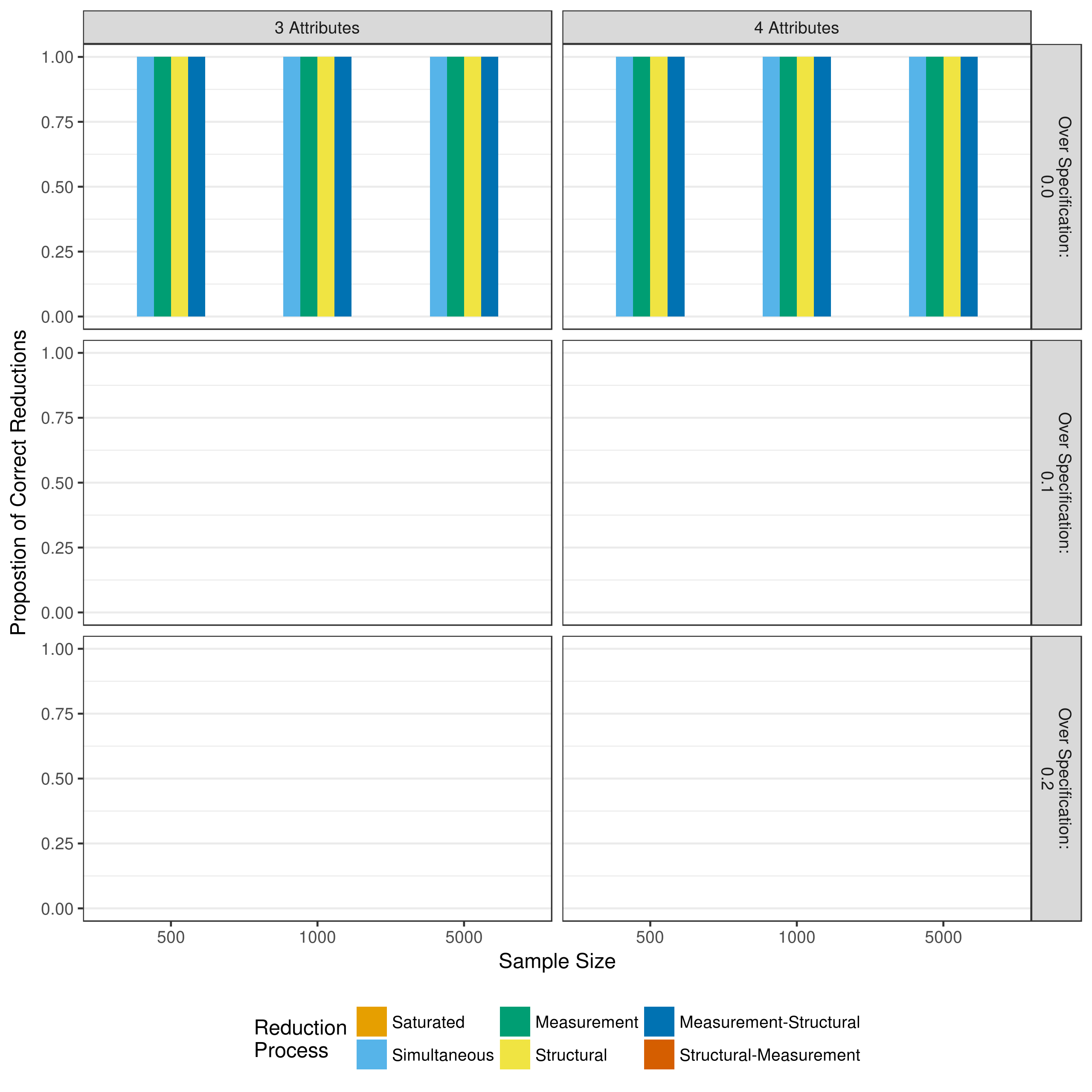
Figure 5.29: Proportion of correct measurement model reductions when reducing with a heuristic
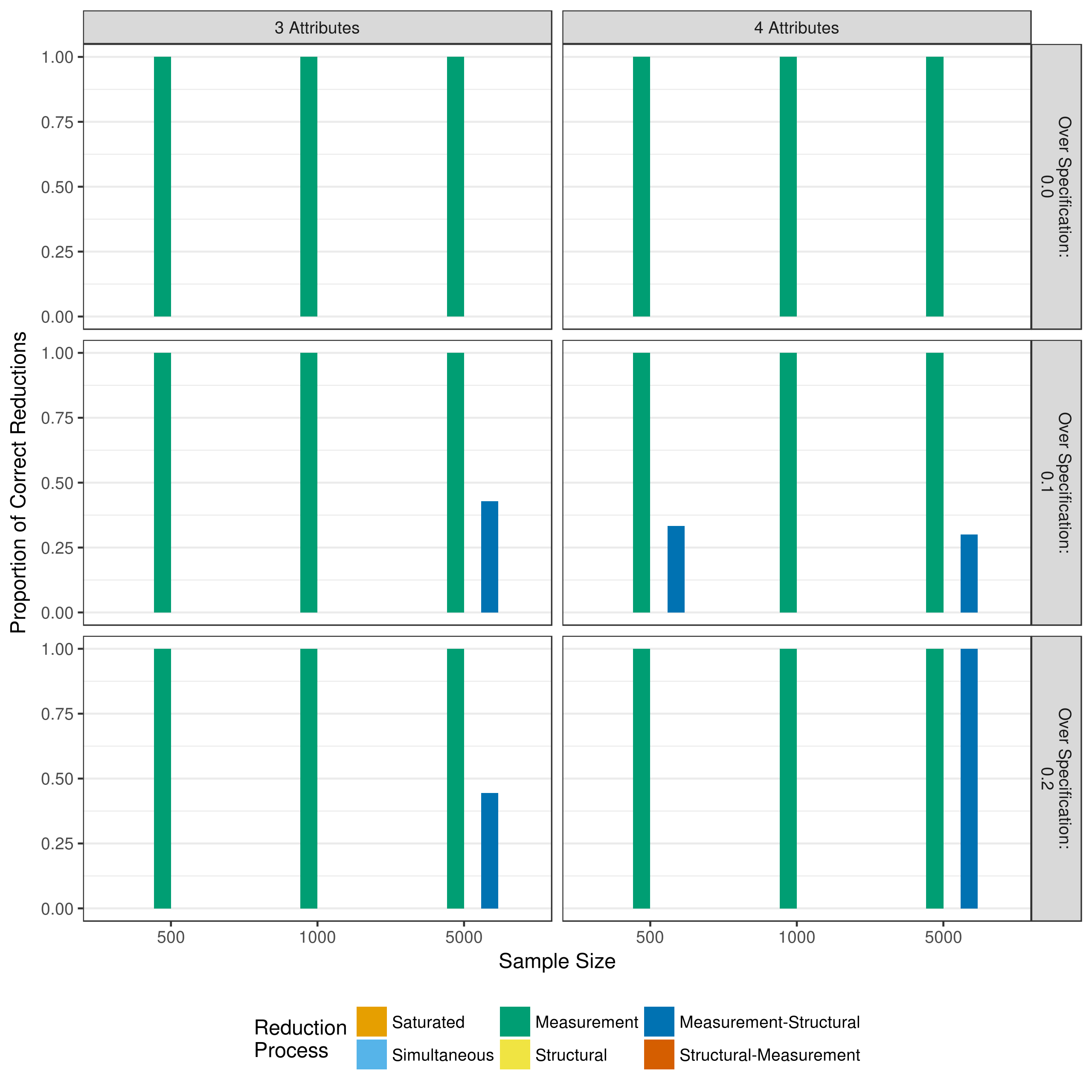
Figure 5.30: Proportion of correct structural model reductions when reducing with a heuristic
Figure 5.29 shows that the only cases where the correct measurement model was obtained was when it was correctly specified, and no parameters were removed using p-values (i.e., simultaneous, measurement, structural, or measurement-structural reduction). However, this should be interpreted with caution. When the Q-matrix is correctly specified, there are no three- and four-way interactions, thus, the heuristic has no parameters to remove. When the Q-matrix is over-specified, removing three- and four-way interactions does nothing to fix the additional main effects that have been added to the model.
Additionally, Figure 5.30, shows that the structural model most usually only correct when only the measurement model was reduced. This is because the data was always generated with a fully saturated structural model. Thus, any removal of parameters (including three- and four-way interactions) results in an incorrect final model.